Visualizing low-level geometric data in Blender

The library provides some utilities to directly visualize low-level representations of geometric objects. This can be useful when you want to visualize something that is not a data structure of the library. Note that this is also what is used under the hood to visualize these data structures.

from ddg.visualization.blender.curve import curve, curve_object
from ddg.visualization.blender.mesh import mesh, mesh_object
from ddg.visualization.blender.object import blender_object, link

Let’s setup a Blender scene:

import bpy
import numpy as np
import ddg.visualization.blender.collection as collection

collection.collection("collection")

Meshes

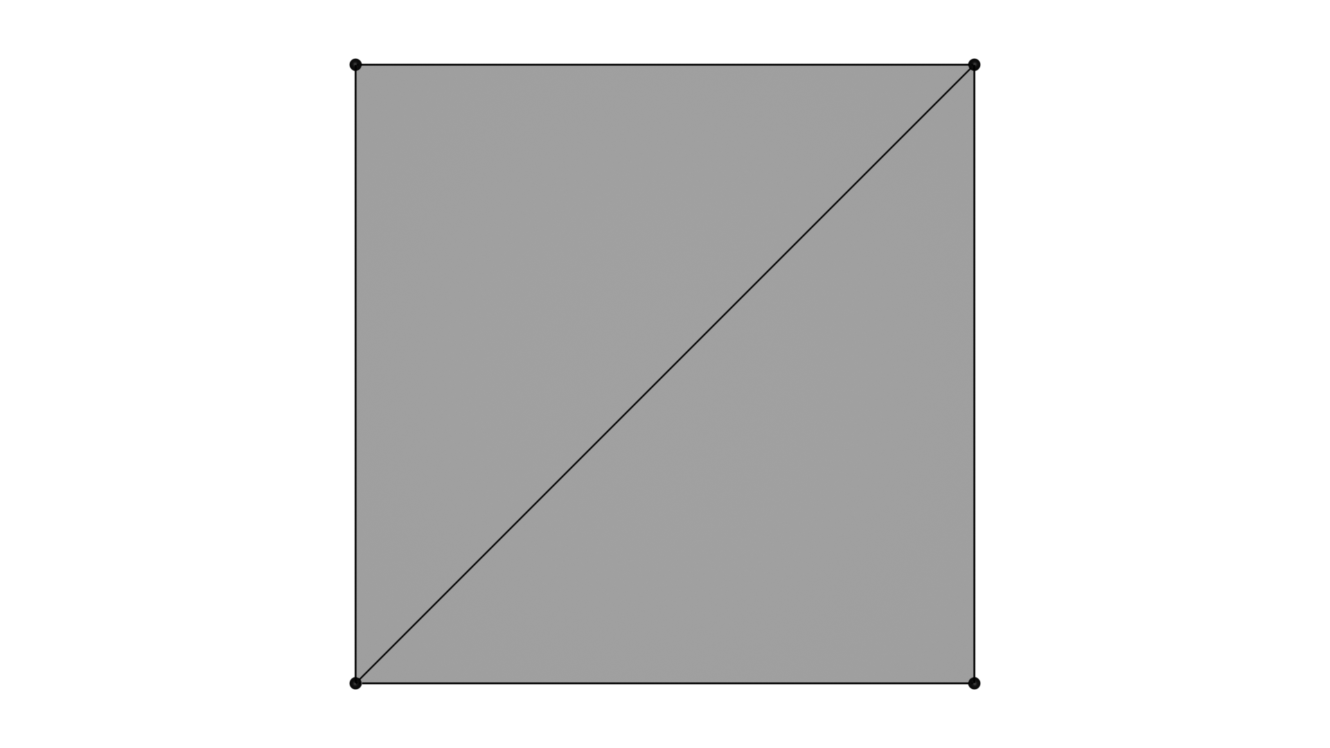
A mesh can be represented as a set of vertices and a set of faces. This is called an indexed face set. Our library provides a very powerful version of IFS, but for sole visualization purposes, having a set of vertices and a set of faces is enough.

# A square divided into two triangles
mesh_points = np.array([(0, 0, 0), (1, 0, 0), (1, 1, 0), (0, 1, 0)])
faces = np.array([(0, 1, 2), (0, 2, 3)])

To visualize this object, one can go step by step, creating a Blender mesh, adding it to a Blender object and linking this object to a collection of the scene:

# Manual version
me = mesh("mesh", mesh_points + np.array((4, 0, 0)), faces)
mesh_bobj_1 = blender_object("manually converted mesh object", me)
link(mesh_bobj_1, "collection")

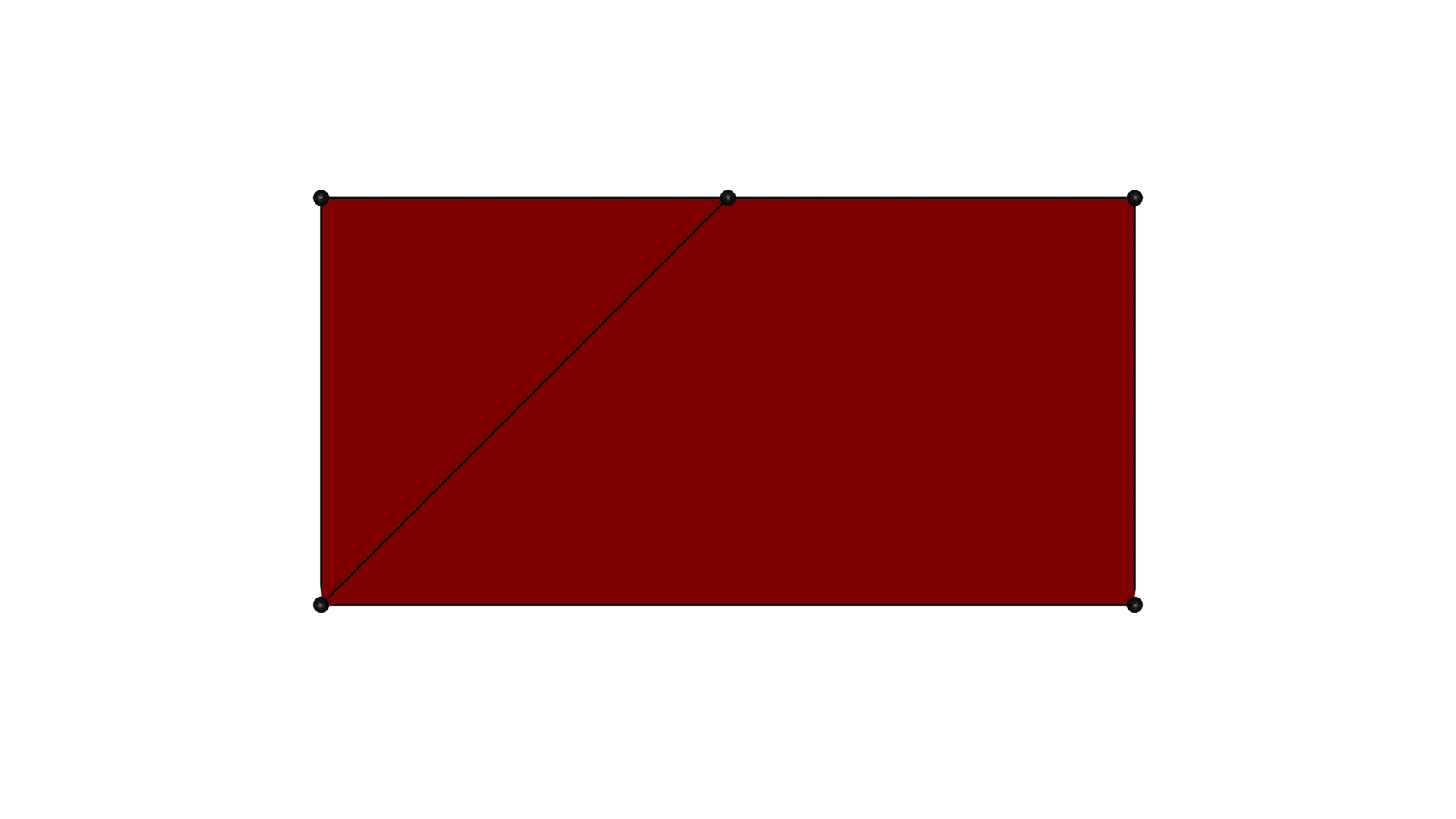
One can also apply arbitrary transformations on the mesh to satisfy the visualization purposes:

import ddg.visualization.blender.mesh as ddg_mesh
import ddg.visualization.blender.bmesh as ddg_bmesh
import ddg.visualization.blender.material as material
from examples.blender.docs.material import mat


def mesh_bobj_transformation(bobj):
    ddg_mesh.shade_smooth(bobj.data)
    with (
        context.mode(bobj, mode="OBJECT"),
        ddg_bmesh.bmesh_from_mesh(bobj.data) as bm,
    ):
        ddg_bmesh.cut_half_space(bm, np.array([0, 1, 0]), 0.5)
    material.set_material(bobj, mat)


mesh_bobj_transformation(mesh_bobj_1)

The steps of the conversion can be reduced to one step by using mesh_object()

# prototype API version
mesh_bobj_2 = mesh_object(mesh_points, faces, "mesh object", "collection")
mesh_bobj_transformation(mesh_bobj_2)

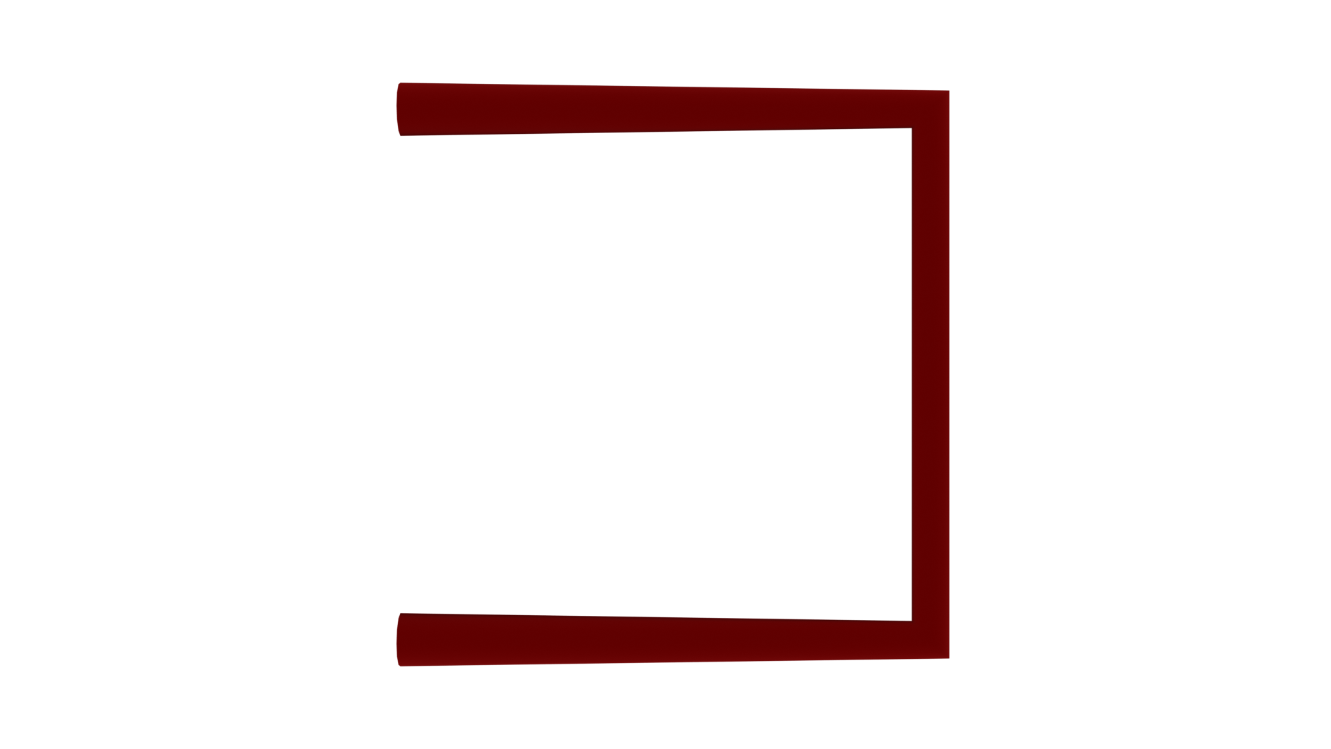
Curves

Similarly curves can be represented as a set of points.

curve_points = np.array([(0, 0, 0), (1, 0, 0), (1, 1, 0), (0, 1, 0)])

Again one can go step by step, creating a Blender curve, adding it to a Blender object and linking this object to a collection of the scene. The noticeable difference here is that the periodicity of the curve is not encoded directly in the set of points, so it needs to be specified additionally when converting:

# Manual version
curve = curve("manually converted curve object", curve_points - 4, False)
curve_object_1 = blender_object(None, curve)
link(curve_object_1, "collection")

One can also apply arbitrary transformations on the curve to satisfy the visualization purposes:

def curve_bobj_transformation(bobj):
    bobj.data.bevel_depth = 0.05
    material.set_material(bobj, mat)


curve_bobj_transformation(curve_object_1)

The steps of the conversion can be reduced to one step by using curve_object()

# prototype API version
curve_object_2 = curve_object(
    curve_points - 2, False, ("curve", "curve object"), "collection"
)
curve_bobj_transformation(curve_object_2)