Nets

Nets are one of our data structures. They represent maps from subdomains of \(\mathbb{R}^m\) or \(\mathbb{Z}^m\) into another space \(X\), e.g. parameterized curves or surfaces. In most cases we will consider maps to \(\mathbb{R}^3.\) There are different types of nets that all inherit from the Net class, for example

• EmptyNet

• PointNet

smooth nets as

• SmoothNet

• SmoothCurve

or their discrete analogs

• DiscreteNet

• DiscreteCurve

• SamplingNet

Further there is the NetCollection class that can handle collections of multible nets.

Smooth nets

Creating a smooth net

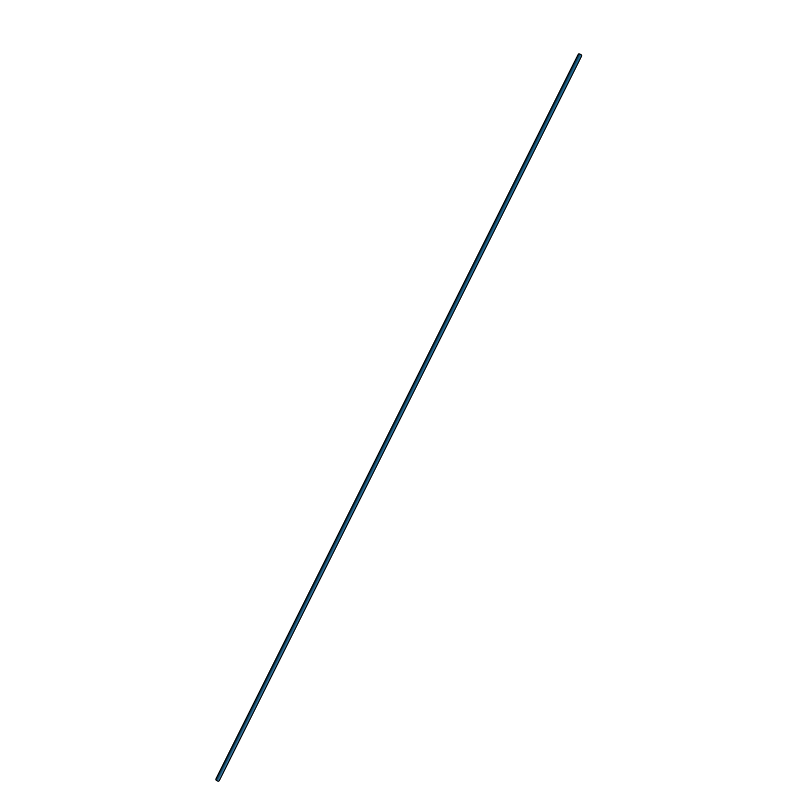
After creating a domain, we can begin constructing a net. For this we only need to define the desired function and pass both, the function and the domain, to the class SmoothNet.

>>> import ddg
>>> import numpy as np

>>> domain = ddg.nets.SmoothDomain([[-4, 4]])
>>> def net_fct(t):
...     return np.array([t, 2*t, 0])

>>> net = ddg.SmoothNet(net_fct, domain)
>>> net(0)
array([0, 0, 0])
>>> net(2)
array([2, 4, 0])

Note

As opposed to a DiscreteNet, a SmoothNet does not store values that have been computed once. The function of a SmoothNet is evaluated anew each time the net is called with some point from the domain.

A short hand to create a domain on the fly you can use the following convention:

>>> import ddg
>>> import numpy as np

>>> def net_fct(t):
...     return np.array([t, 2*t, 0])

>>> net = ddg.SmoothNet(net_fct, [[-4, 4]])
>>> net(0)
array([0, 0, 0])
>>> net(2)
array([2, 4, 0])

Note that similar to SmoothDomain, SmoothNet expects a list of intervals when the domain is passed in this way. Similar to SmoothInterval there is the class SmoothCurve which lifts this restriction.

Further Examples

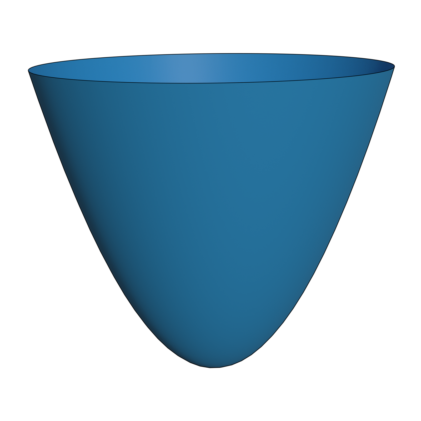
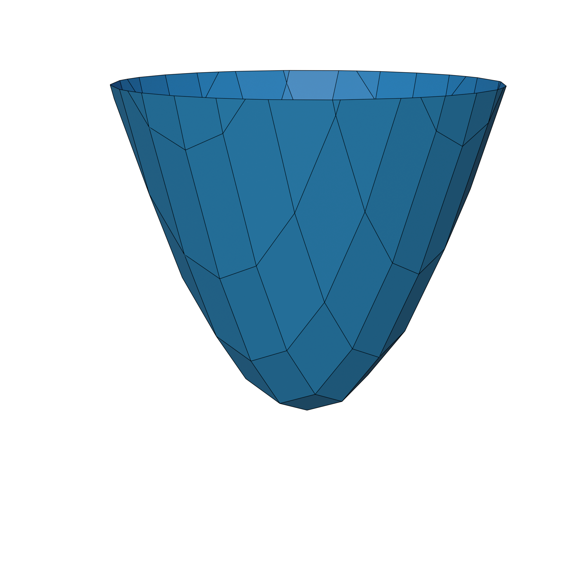
Example: Paraboloid

>>> import ddg

>>> domain = ddg.nets.SmoothDomain([[-4, 4], [-4, 4]])
>>> def paraboloid_fct(x,y):
...     return (x, y, x**2 + y**2)

>>> paraboloid_net = ddg.SmoothNet(paraboloid_fct, domain)

Example: Helix

>>> import ddg
>>> import numpy as np

>>> def helix_fct(t):
...     return (np.cos(t), np.sin(t), t)

>>> helix_net = ddg.SmoothNet(helix_fct, [[-2*np.pi, 2*np.pi]])

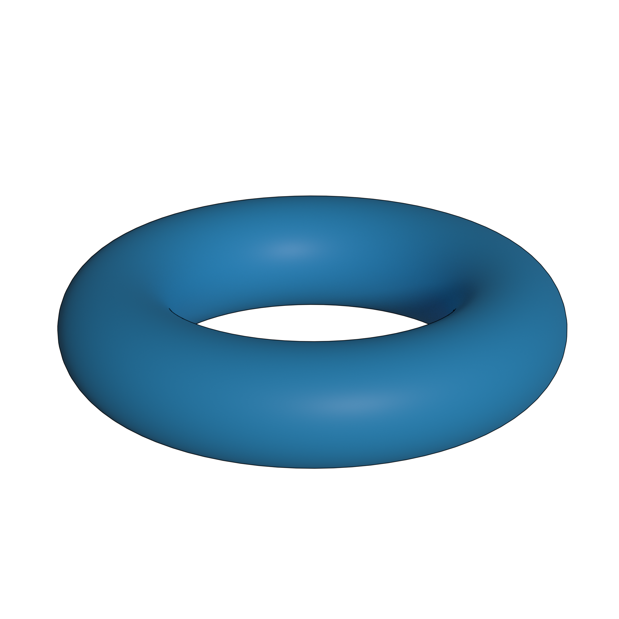
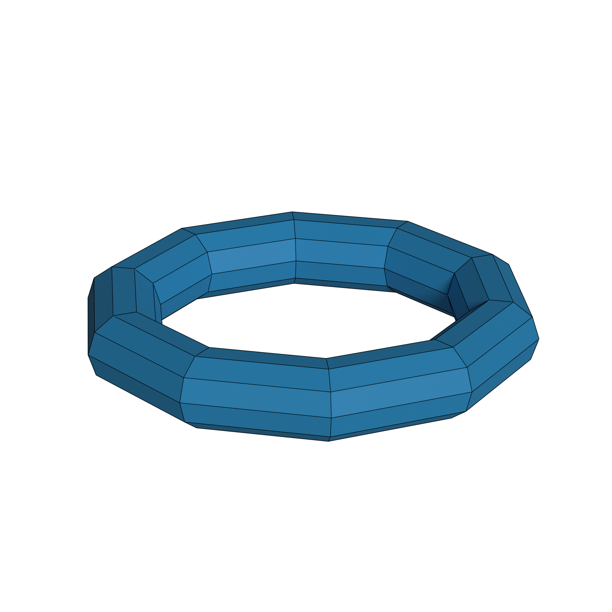
Example: Torus

>>> import ddg
>>> import numpy as np

>>> def torus_fct(u,v):
...     a = 0.2
...     b = 1
...     x1 = (a*np.cos(u)+b)*np.cos(v)
...     x2 = (a*np.cos(u)+b)*np.sin(v)
...     x3 = a*np.sin(u)
...     return (x1, x2, x3)

>>> torus_net = ddg.SmoothNet(torus_fct, [[0, 2*np.pi, True],[0, 2*np.pi, True]])

Discrete nets

When we want to visualize our net in Blender, we have to make sure that we pass discrete information to it. For this we use DiscreteNet. All in all, the process of creating a discrete net is not any different from creating a smooth one - we could just replace most instances of “Smooth” with “Discrete” - but we have to make sure that our domain is a subset of \(\mathbb{Z}^n\). Though it is still possible to evaluate the net at any given “real” point, only the integer points of the domain will be used further, e.g. for the visualization in Blender.

Creating a discrete net

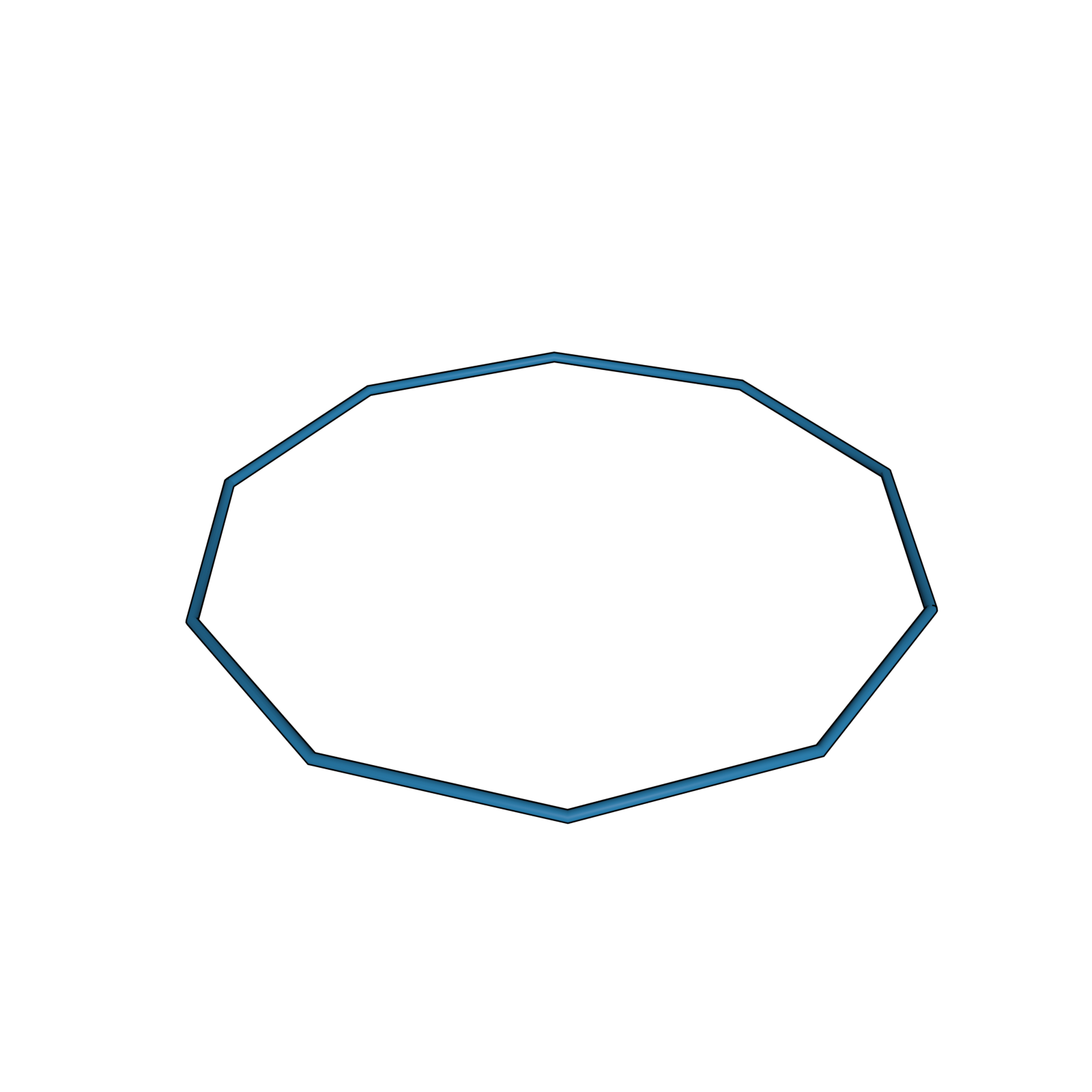
The process of creating a discrete net mirrors the smooth case, but we have to take care of mapping our discrete domain to not only valid, but also “reasonable” real points to achieve our desired result. Similar the smooth case the DiscreteDomain can be created on the fly as in the following where we will create a discrete net of a circle with 10 points in the domain. (One can also explicitly create discrete domains.)

>>> import ddg
>>> import numpy as np

>>> def discrete_circle_fct(n):
...     t = 2*np.pi/10*n
...     return np.array([np.cos(t), np.sin(t), 0])

>>> discrete_circle = ddg.DiscreteNet(discrete_circle_fct, [[0, 9, True]])
>>> discrete_circle(0)
array([1., 0., 0.])

You might have noticed that we never reach the value \(t=2\pi\) in the function above. This is by design as the net is periodic.

Warning

As opposed to a SmoothNet, a DiscreteNet saves every value after it has been computed once. If you call a DiscreteNet with the same point from the domain a second time the saved value is returned.

Further examples

The following examples will show you how you could create discrete nets corresponding to the examples given for smooth nets.

Example: Paraboloid

>>> import ddg

>>> def discrete_paraboloid_fct(x,y):
...     x /= 2.5
...     y /= 2.5
...     return (x, y, x**2 + y**2)

>>> discrete_paraboloid = ddg.DiscreteNet(discrete_paraboloid_fct, [[-10, 10]]*2)

Example: Helix

>>> import ddg
>>> import numpy as np

>>> def discrete_helix_fct(t):
...     t = -2*np.pi + t
...     return (np.cos(t), np.sin(t), t)

>>> discrete_helix = ddg.DiscreteNet(discrete_helix_fct, [[0, 11]])

Example: Torus

>>> import ddg
>>> import numpy as np

>>> def discrete_torus_fct(u,v):
...     a = 0.2
...     b = 1
...     s = 2*np.pi/10
...     u = u*s
...     v = v*s
...     x1 = (a*np.cos(u)+b)*np.cos(v)
...     x2 = (a*np.cos(u)+b)*np.sin(v)
...     x3 = a*np.sin(u)
...     return (x1, x2, x3)

>>> discrete_torus = ddg.DiscreteNet(discrete_torus_fct, [[0, 9, True],[0, 9, True]])

The process of converting smooth nets to discrete nets in this fashion is rather tedious. We will go over a different way to achieve this conversion later.

Net collections

Sometimes an object can not be represented by a single net, but we want to consider multiple nets as one. as one. For this we have the Netcollection class.

Net collections are exactly what the name describes: a collection of nets.

>>> import ddg
>>> import numpy as np

>>> def line_fct_1(t):
...     return np.array([t, t, 0])
>>> def line_fct_2(t):
...     return np.array([t, -t, 0])

>>> line1 = ddg.SmoothNet(line_fct_1, [[-4, 4]])
>>> line2 = ddg.SmoothNet(line_fct_2, [[-4, 4]])

>>> crossing_lines = ddg.NetCollection([line1, line2])

In the utils module of nets we can find the definition of a applicable_to_netcollection() decorator. Any function decorated by it will always be able to be applied to both nets and net collections.

Example: Double helix

>>> import ddg
>>> import numpy as np

>>> def helix_fct_1(t):
...     return (np.cos(t), np.sin(t), t)

>>> def helix_fct_2(t):
...     return (np.cos(t+np.pi), np.sin(t+np.pi), t)

>>> helix_net_1 = ddg.SmoothNet(helix_fct_1, [[-2*np.pi, 2*np.pi]])
>>> helix_net_2 = ddg.SmoothNet(helix_fct_2, [[-2*np.pi, 2*np.pi]])

>>> double_helix = ddg.NetCollection([helix_net_1, helix_net_2])

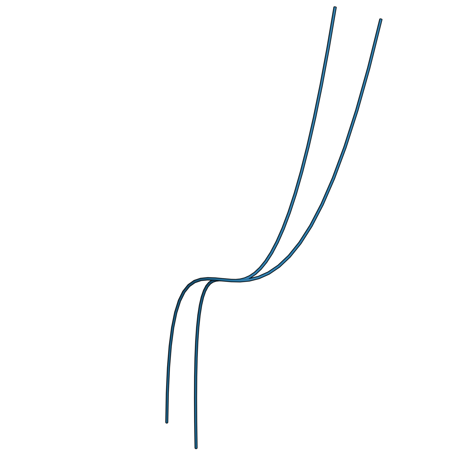
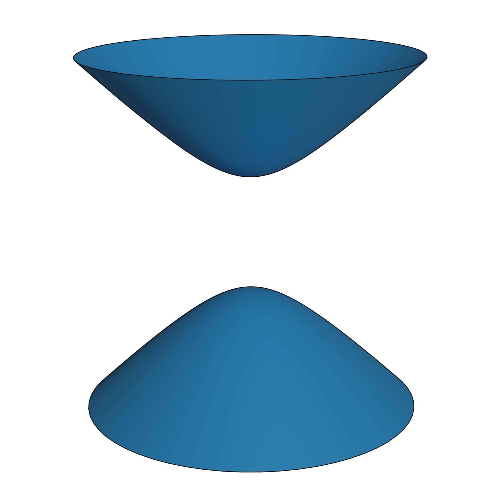
Example: Two-sheeted hyperboloid

>>> import ddg
>>> import numpy as np

>>> def first_sheet_fct(u, v):
...     return (np.sinh(u)*np.cos(v), np.sinh(u)*np.sin(v), np.cosh(u))
>>> def second_sheet_fct(u, v):
...     return (np.sinh(u)*np.cos(v), np.sinh(u)*np.sin(v), -np.cosh(u))

>>> first_sheet = ddg.SmoothNet(first_sheet_fct, [[0, np.inf],[0, 2*np.pi, True]])
>>> second_sheet = ddg.SmoothNet(second_sheet_fct, [[0, np.inf],[0, 2*np.pi, True]])

>>> two_sheeted_hyperboloid = ddg.NetCollection([first_sheet, second_sheet])
>>> two_sheeted_hyperboloid.transform(np.diag([1,2,1]))

Modifying nets

We do not have to be done with our nets once we have created them. In the following we will go over two ways of modifying or creating new nets from old ones.

Transformations

The net classes inherit from the class Transformable. As such it contains a transformation stack on which we can push any functions or matrices which are able to transform points from the target space of our function.

>>> import ddg
>>> import numpy as np

>>> net = ddg.SmoothNet(lambda t: np.array([t, t**2, t**3]), [[-np.inf, np.inf]])
>>> net(2)
array([2, 4, 8])

>>> net.transform(np.diag([1/2, 1/2, 1/2]))
>>> net(2)
array([1., 2., 4.])

Note that transformations always act in-place, i.e. the values of the net will change.

In the utils module of nets you can find the three functions embed, homogenize and dehomogenize which are applied to a net, but change the transformation stack.

>>> import ddg
>>> import numpy as np

>>> net = ddg.SmoothNet(lambda t: np.array([np.cos(t), np.sin(t)]), [[0, np.pi, True]])
>>> net(0)
array([1., 0.])

>>> ddg.nets.utils.embed(net)

>>> net(0)
array([1., 0., 0.])

>>> net.pop_transformation()
<function embed.<locals>.<lambda> at 0x...>

>>> ddg.nets.utils.homogenize(net)
>>> net(0)
array([1., 0., 1.])

>>> ddg.nets.utils.dehomogenize(net)
>>> net(0)
array([1., 0.])

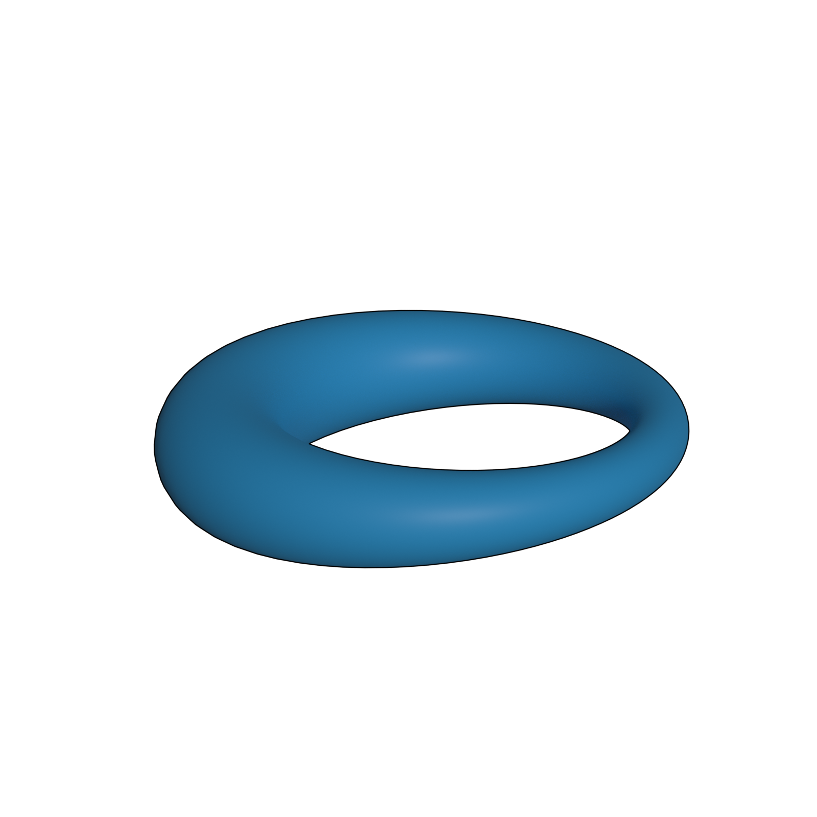
Example: Torus inverted in a unit sphere

>>> import ddg
>>> import numpy as np

>>> def torus_fct(u,v):
...     a = 0.2
...     b = 1
...     x1 = (a*np.cos(u)+b)*np.cos(v)
...     x2 = (a*np.cos(u)+b)*np.sin(v)
...     x3 = a*np.sin(u)
...     return np.array((x1, x2, x3))

>>> torus_net = ddg.SmoothNet(torus_fct, [[0, 2*np.pi, True],[0, 2*np.pi, True]])

>>> translation = lambda x: np.array([x[0]+0.2, x[1], x[2]])
>>> inversion = lambda x: x/sum([i**2 for i in x])

>>> torus_net.transform(translation)
>>> torus_net.transform(inversion)

Utility functions

Another way of working with nets is the to use our utility functions on them. While domain utility functions will create, when you pass them an actual domain, they will replace the domain of a given net instead.

>>> import ddg
>>> import numpy as np

>>> net = ddg.SmoothNet(lambda t: t, [[-np.inf, np.inf]])
>>> net.domain.intervals
[[-inf, inf]]

>>> new_net = ddg.nets.utils.bound_domain(net, 10)
>>> new_net is net
True

>>> new_net.domain.intervals
[[-5.0, 5.0]]

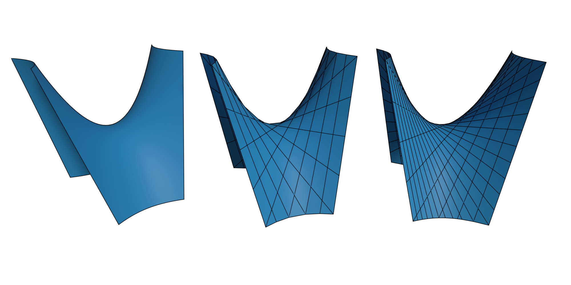
Example: Surface of revolution

>>> import ddg
>>> import numpy as np

>>> hyperbola1 = lambda u: np.array([np.sinh(u), np.cosh(u)])
>>> hyperbola2 = lambda u: np.array([np.sinh(u), -np.cosh(u)])

>>> hyperbola1 = ddg.SmoothNet(hyperbola1, [[0, np.inf]])
>>> hyperbola2 = ddg.SmoothNet(hyperbola2, [[0, np.inf]])

>>> hyperbola1 = ddg.nets.utils.surface_of_revolution(hyperbola1)
>>> hyperbola2 = ddg.nets.utils.surface_of_revolution(hyperbola2)

>>> two_sheeted_hyperboloid = ddg.NetCollection([hyperbola1, hyperbola2])

More utility functions

The utils module of nets contains a collection of utility functions which can be applied to nets. An example is coordinate_lines() , which returns a NetCollection of curves describing the coordinate lines of the discrete net.

Sampling a smooth net

When we were talking about discrete nets, we have seen ways on how to convert a smooth net into a discrete one.

Since this process is usually the same, our library provides the function sample_smooth_net to automate this process.

>>> import ddg
>>> import numpy as np

>>> net = ddg.SmoothNet(lambda x,y: np.array([x, y, x*y]), [[-5, 5]]*2)
>>> discrete_net = ddg.sample_smooth_net(net, 0.5)
>>> discrete_net.domain.intervals
[[0, 20], [0, 20]]
>>> (discrete_net(0,0) == net(-5, -5)).all()
True

The above example shows how to use the defaulting option for sample_smooth_net. We can also pass on samplings for each direction of our domain.

>>> import ddg
>>> import numpy as np

>>> net = ddg.SmoothNet(lambda x,y: np.array([x, y, x*y]), [[-5, 5]]*2)
>>> discrete_net = ddg.sample_smooth_net(net, [0.5, 0.2])
>>> discrete_net.domain.intervals
[[0, 20], [0, 49]]
>>> discrete_net(10, 49)
array([0. , 4.8, 0. ])

We can choose between different sampling options for each direction of our domain.

The following table shows the available options for sampling a smooth net. It contains whether an option can be used for a bounded/unbounded direction, of what type the argument has to be, and whether it can or does preserve the periodicity of the direction.

The general form of a sampling has to be [sample, option] with the exceptions of compound (passed as: [stepsize, total-amount, 'c']) and stepsize (can be passed as stepsize without any brackets) sampling.

options	‘’	‘t’	‘c’	‘s’
meaning	stepsize	total	compound	symmetric
bounded	yes	yes	yes	yes
unbounded	yes	no	yes	no
type	float	int	float, int	float
periodic	can preserve	preserves	preserves	can preserve

For example we could find it easier to use the total option to specify the sampling of a bounded direction:

>>> import ddg
>>> import numpy as np

>>> net = ddg.SmoothNet(lambda x,y: np.array([x, y, x*y]), [[-5, 5]]*2)
>>> discrete_net = ddg.sample_smooth_net(net, [10, 't'])
>>> discrete_net.domain.intervals
[[0, 9], [0, 9]]

>>> discrete_net = ddg.sample_smooth_net(net, [[10, 't'], [5, 't']])
>>> discrete_net.domain.intervals
[[0, 9], [0, 4]]

>>> discrete_net = ddg.sample_smooth_net(net, [0.5, [5, 't']])
>>> discrete_net.domain.intervals
[[0, 20], [0, 4]]

Note that giving a total amount of samples for an unbounded direction does not make sense. Thus only the stepsize option can be used in that case.

>>> import ddg
>>> import numpy as np

>>> net = ddg.SmoothNet(lambda x,y: np.array([x, y, x*y]), [[-np.inf, np.inf]]*2)
>>> discrete_net = ddg.sample_smooth_net(net, 0.1)
>>> discrete_net.domain.intervals
[[-inf, inf], [-inf, inf]]

Sometimes we are not sure what kind of domain our given net has and we want to specify both a stepsize and a total amount of samples for it. We call this compound sampling.

When the direction is bounded, the total number of samples will be used, while for unbounded directions the stepsize is used instead.

>>> import ddg
>>> import numpy as np

>>> net = ddg.SmoothNet(lambda x,y: np.array([x, y, x*y]), [[-np.inf, np.inf]]*2)
>>> discrete_net = ddg.sample_smooth_net(net, [0.5, 10, 'c'])
>>> discrete_net.domain.intervals
[[0, 9], [0, 9]]

Note how we obtained a bounded domain eventhough we sampled an unbounded one. The total amount given in the compound sampling will be used to bound the domain similar to the utility function bound_domain.

The SamplingNet class

In our net module we find another type of net which we haven’t discussed yet. A sampling net is a special kind of a discrete net created in the sampling process. It contains the sampling functions, which map our discrete to our smooth domain.

It is a discrete net whose function can fundamentally change through updates caused by our update graph (e.g. change of parameters).

Conversion to halfedge

Nets of dimension 2 or less with bounded domains can be converted to a The half-edge data structure object using the function ddg.conversion.halfedge.nets.discrete_net_to_halfedge(). The vertices of the resulting half-edge object will have an attribute "co" containing the value of the net at that point and the order will be the same as that in the traverser of the domain.

>>> from ddg.conversion.halfedge.nets import discrete_net_to_halfedge
>>> def f(x, y):
...     return np.array([x, y, x**2 - y**2])
...
>>> net = ddg.DiscreteNet(f, [[0, 1], [0, 1]])
>>> surface = discrete_net_to_halfedge(net)

>>> for c in net.traverser:
...     print(net[c])
[0 0 0]
[ 0  1 -1]
[1 0 1]
[1 1 0]

>>> for v in surface.verts:
...     print(v.co)
[0 0 0]
[ 0  1 -1]
[1 0 1]
[1 1 0]

The name of the coordinate attribute can be changed using the co_attr argument of the conversion function.

Visualization in Blender

A guide on how to visualize ddg objects, including nets can be found here .