Visualizing ddg objects in blender

Note

First steps on how to run a script in Blender can be found here.

Everything that deals with the visualization of ddg objects in Blender is located in the package ddg.conversion.blender. All that is needed for such a conversion is the function to_blender_object(), located at ddg.conversion.blender.core. For convenience there also exists a helper function to_blender_object_helper() that helps with passing commonly used arguments in an easy way and, if needed, wrapping some object conversions. One can use either of those functions for the conversion to blender. Generally the second function helps with preparing objects for the conversion but in the end it calls to_blender_object() itself for the conversion.

Currently the following types are directly convertible to blender:

• EmptyNet

• PointNet

• DiscreteNet

• DiscreteCurve

• NetCollection

• Surface

Other objects, e. g. geometric objects or SmoothNet have to be converted to one of the above and thus can not be given to to_blender_object() directly. This can be done manually (e.g. to a SmoothNet and then to a DiscreteNet) or they can be handed to to_blender_object_helper(). For the conversion some additional conversion arguments might be required. The only conversion supported by to_blender_object_helper() until now is via SmoothNet and then to a DiscreteNet where the last conversion requires a sampling keyword, like sampling=[.1, 50, 'c'] (For more information on sampling see here: Nets). Aside from that all conversions can be customized with a great variety of keyword arguments (see api docs of to_blender_object_helper()).

Usage of ddg.to_blender_object and ddg.to_blender_object_helper

The usage of to_blender_object() is straight forward (no extra conversion/sampling needed in this example):

>>> import ddg
>>> from ddg.datastructures.halfedge.surface_generator import cube
>>> cube = cube()
>>> blender_object = ddg.to_blender_object(cube)

We will firstly investigate the signature of to_blender_object():

>>> to_blender_object(obj, attributes={},
...                        mesh_transformations=[], bmesh_transformations=[], obj_transformations=[],
...                        material=None, collection=None, accept_all=False, depth_bounding=10,
...                        **options)

Possible keyword arguments can be distinguished by the following types for which the most important examples are given:

• attributes of the blender object

  • name

  • location

  • hide_viewport

  • hide_render

  • scale

• transformations of the mesh

  • shade_smooth()

• transformations of the bmesh

  • cut_bounding_box()

• transformations of the blender object

• others as accept_all=False, depth_bounding=10, material=None, collection=None

• special options depending on the given object

The arguments name, hide_viewport, hide_render and location are arguments that can simply be set as attributes of the resulting blender object. Therefore they get passed on to the attributes dictionary that is handed to the conversion function. Transformations on meshes, bmeshes and blender objects can be given as lists of transformation functions (or as a single function if only on was given). These functions require precisely one argument: the mesh, bmesh or blender object, respectively. The utility function cut_bounding_box() cuts objects within the given dimensions of a box to obtain clean borders for visualization. The mesh transformation shade_smooth() simplifies the rendering process of smooth surfaces. A full documentation of the keyword arguments can be found in the api documentation of to_blender_object().

When working on a larger script with multiple objets to convert to blender it quickly becomes clear that explicitly stating all desired keyword arguments in such a way in each function call is quite inconvenient. Therefore the to_blender_object_helper() is what to use in practice. It’s signature reads

>>> to_blender_object_helper(obj,
...                   name=None, location=None, hide_viewport=True, hide_render=True, scale=(1,1,1),
...                   shade_smooth=False, bounding_box=None,
...                   material=None, collection=None, accept_all=False,
...                   **kwargs)

The **kwargs may contain any further keyword arguments that will directly be passed over to to_blender_object(). If, e.g. mesh transformations are given as a list and simultaneously shade_smooth=True, the list of mesh transfomation will be extended by the mesh transformation that does the smooth shading and the combined list will be handed over to to_blender_object(). As an example the two function calls shown below will yield the same result. We use a quadric as an example object.

>>> import numpy as np
>>> import ddg
>>> cone = ddg.geometry.quadrics.Quadric(np.diag([2, 3, -1, 0]))

Using to_blender_object():

>>> snet_cone = ddg.to_smooth_net(cone, affine=True)
>>> dnet_cone = ddg.sample_smooth_net(snet_cone, sampling=[.1, 20, 'c'])
>>> bmesh_trafo = lambda bmesh: ddg.visualization.blender.bmesh.cut_bounding_box(bmesh, [3,3,3])
>>> mesh_trafo = ddg.visualization.blender.mesh.shade_smooth
>>> blender_object = ddg.to_blender_object(dnet_cone,
...                                    attributes={'name':'cone', 'location':(1,1,1)},
...                                    mesh_transformations=mesh_trafo, bmesh_transformations=bmesh_trafo,
...                                    only_wire=True)

and using to_blender_object_helper()

>>> blender_object = ddg.to_blender_object_helper(cone, sampling=[.1,20,'c'],  name='cone', location=(1,1,1), bounding_box=[3,3,3],
...                                               shade_smooth=True, only_wire=True)

Visualizing half-edge objects

Half-edge objects to not require any further conversion and can be visualized directly, providing the vertices have an attribute that stores the coordinates. The default name of this attribute is "co". It can be specified in the to_blender_object_helper() (to_blender_object()) function call:

>>> import ddg
>>> cube = ddg.halfedge.surface_generator.cube()

>>> bobj = ddg.to_blender_object(cube, co_attr='co')
>>> bobj = ddg.to_blender_object_helper(cube, co_attr='co')

Tubes and Spheres

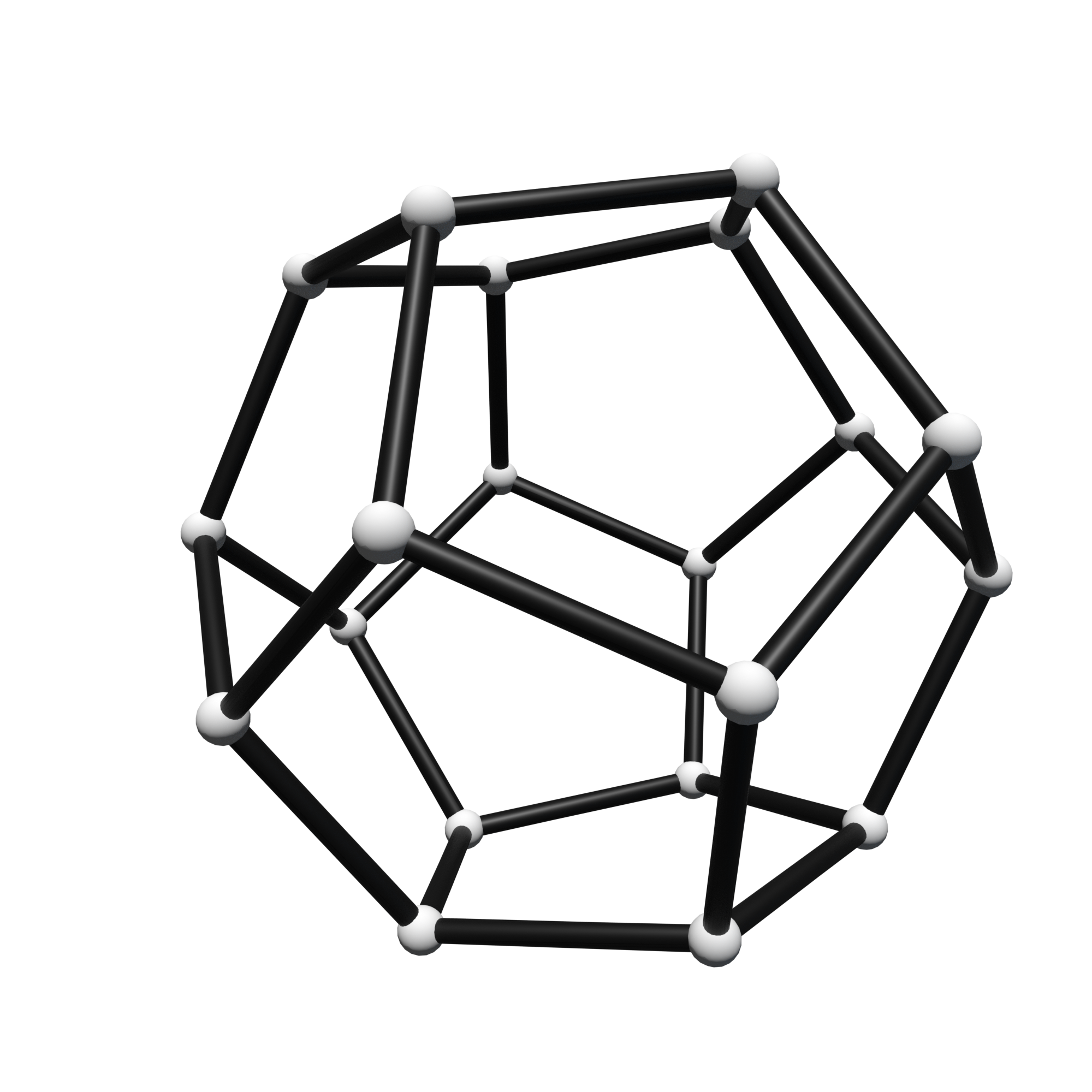
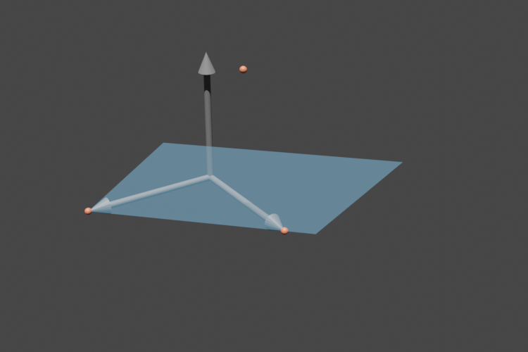
Next to the standard conversion to blender, for half-edge objects there exists a function hes_to_tubes_and_spheres_blender_object() that converts a half-edge object to an empty Blender object that functions as a parent object for cylinders representing the edges and spheres representing the vertices. By default the name of the vertex attribute of the initial half-edge object storing the coordinates is "co". The function hes_to_tubes_and_spheres_blender_object() also allows adaption of the cylinders and spheres as keyword arguments (see also in the half-edge users guide). Further it has the keyword arguments parent_kwargs={}, kwargs_generator=None. The first one, parent_kwargs, is a dictionary handed over to to_blender_object() that allows modification of the empty parent object. The second one, kwargs_generator is either a None or a function. This function takes a cell and returns a dictionary of keyword arguments supplied to to_blender_object() when visualizing the cell as a cylinder or a sphere:

>>> dodecahedron = ddg.halfedge.surface_generator.dodecahedron()

>>> def kwargs_generator(cell):
...     hds = cell.surf
...     if type(cell) is hds.verts:
...         material = 'white'
...     elif type(cell) is hds.edges:
...         material = 'black'
...     kwargs = {'material': material, 'attributes':{'location':[0,5,0]} }
...     return kwargs

>>> bobj = ddg.conversion.blender.halfedge.hes_to_tubes_and_spheres_blender_object(dodecahedron, co_attr='co',
...                                        tube_resolution=30, fill_tube_caps=True, tube_radius=1,
...                                        sphere_subdivision_steps=1, sphere_radius=1,
...                                        parent_kwargs={}, kwargs_generator=kwargs_generator)

Another common example is using the function to visualize the bi-coloring described in the half-edge users guide. for example by

>>> grid = ddg.halfedge.surface_generator.grid(4, 4)

>>> def kwargs_generator_bicoloring(cell, cell_to_color='verts', color_attr='color', kwargs={}):
...   hds = cell.surf
...   if type(cell) is getattr(hds, cell_to_color):
...        material = getattr(cell, color_attr)
...   else:
...       material = 'a_bit_darker_blue'
...   kwargs.update({'material': material})
...   return kwargs

>>> v1, v2 = ddg.halfedge.set.bicolor_vertices(grid, color_attr='color', colors=['black', 'white'], initial_vertex_index=0)
>>> kwargs_generator = lambda cell: kwargs_generator_bicoloring(cell, cell_to_color='verts', color_attr='color', kwargs={})
>>> bobj = ddg.conversion.blender.halfedge.hes_to_tubes_and_spheres_blender_object(grid, kwargs_generator=kwargs_generator)

>>> e1, e2 = ddg.halfedge.set.bicolor_edges(grid, color_attr='color', colors=['black', 'white'], initial_edge_index=0)
>>> kwargs_generator = lambda cell: kwargs_generator_bicoloring(cell, cell_to_color='edges', color_attr='color', kwargs={'attributes': {'location':[5,0,0]}})
>>> bobj = ddg.conversion.blender.halfedge.hes_to_tubes_and_spheres_blender_object(grid, kwargs_generator=kwargs_generator)

Visualizing nets

Given a SmoothNet (or a SmoothCurve), for the conversion to blender it has to be converted to a discrete net first. Therefore a sampling must be given to to_blender_object_helper() or it must be manually be converted to a DiscreteNet (or a DiscreteCurve).

>>> smooth_net = ddg.datastructures.nets.net_generators.spheres_and_circles.circle((0, 0, 0), 1)

>>> blender_object = ddg.to_blender_object_helper(smooth_net, sampling=[0.5, 10, 'c'])

>>> discrete_net = ddg.sample_smooth_net(smooth_net, [0.5, 10, 'c'])
>>> blender_object = ddg.to_blender_object(discrete_net)  

For more information on the sampling see in the documentation of nets.

Depending on the type of the discrete net (DiscreteNet, DiscreteCurve, PointNet), additional arguments can be given to the conversion function:

• DiscreteCurve :

  boundingint (optional, default=10)

  Used to bound unbounded domains of nets.

  curve_typestring (optional, default=’POLY’)

  Blender curve type. See the Blender docs for all available types.

  curve_propertiesdictionary (optional, default={‘bevel_depth’: 0.015})

  Dictionary containing Blender curve properties. See the Blender docs for all available properties.

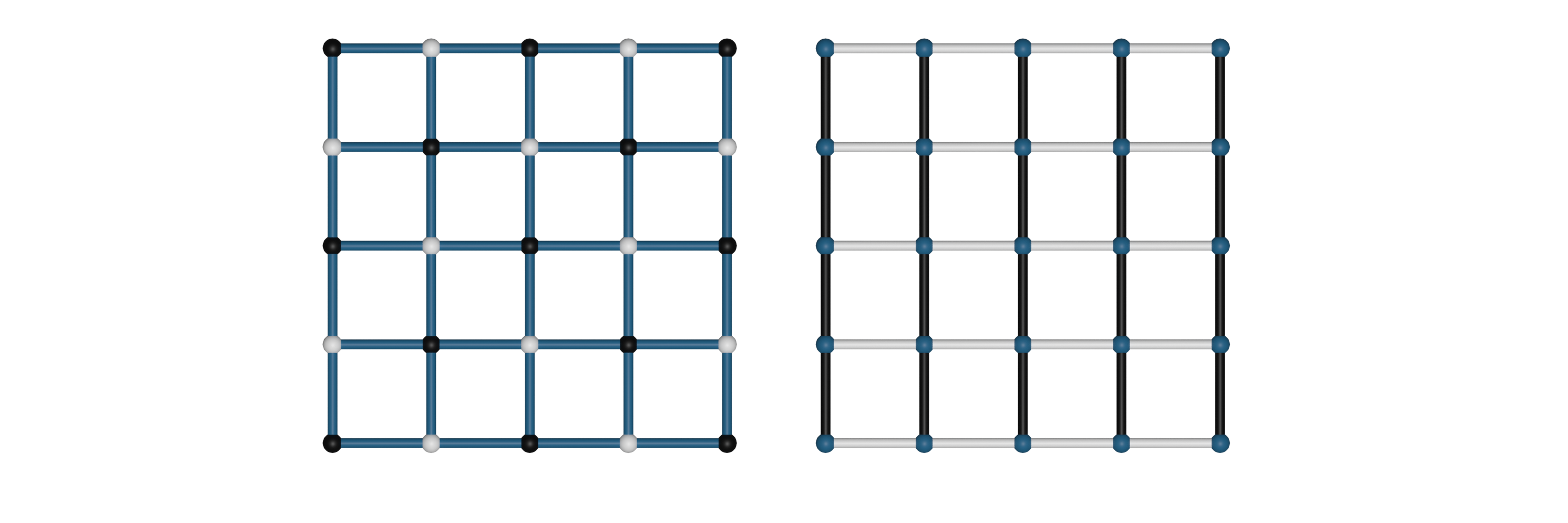
• DiscreteNet :

  only_wirebool (optional, default=False)

  When True, only the wireframe of the net will be created.

• PointNetsphere_radius, sphere_subdivision

  sphere_radiusfloat (optional, default=0)

  Radius of the sphere representing a point.

  sphere_subdivisionint (optional, default=3)

  How many subdivisions will be applied to the sphere.

These arguments are also documented in the to_blender_object() api documentation.

Warning

DiscreteNets and DiscreteCurves are converted to Blender Mesh objects and Blender Curve objects, respectively. Thus these objects have to be handled differently. Particularly mesh and bmesh transformations that can be handed to to_blender_object_helper() as keyword arguments do not work for curves. The desired transformations have to be implemented differently.

For example the bmesh cut_bounding_box() transformation is needed frequently for visualization and therefore a corresponding transformation cut_bounding_box() has been implemented for curves. to_blender_object_helper() internally decides which to use when bounding_box was given.

Visualizing subspaces

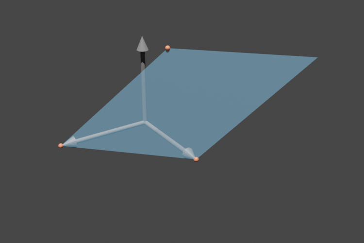
A subspace converted to a SmoothNet can further be converted to a DiscreteNet and then visualized in Blender. For more information on the sampling of nets (used in the conversion to a discrete net) see here.

Note

For conversion to a SmoothNet one can use affine=True and/or convex=True, see also in the users guide of subspaces. to_blender_object_helper() sets both to True by default.

>>> points1 = [[1,0,0,1],[0,1,0,1]]
>>> points2 = [[1,1,0,2],[0,0,1,2]]
>>> subspace1 = ddg.geometry.subspaces.Subspace(*points1)
>>> subspace2 = ddg.geometry.subspaces.Subspace(*points2)

>>> meet = ddg.geometry.subspaces.meet(subspace1, subspace2)
>>> join = ddg.geometry.subspaces.join(subspace1, subspace2)

>>> bobj1 = ddg.to_blender_object(subspace1, sampling=.1, bevel_depth=0.015)  
>>> bobj2 = ddg.to_blender_object(subspace2, sampling=.1, bevel_depth=0.015)  
>>> bobj_join = ddg.to_blender_object(join, sampling=[.1,20,'c']) 
>>> bobj_meet = ddg.to_blender_object(meet, sphere_radius=.05, sphere_subdivision=4) 

Here are some example code snippets and the images they produce. We also drew all points in subspace.points that are not at infinity.

>>> s = ddg.geometry.subspaces.Subspace([1, 0, 0, 1], [0, 0.5, 1, 1])
>>> bobj = ddg.to_blender_object_helper(s, sampling=[.1, 40, 'c'], domain=[[0, 1]])  

>>> s = ddg.geometry.subspaces.Subspace([1, 0, 0, 1], [0, 1, 0, 1], [0, 0.5, 1, 1])
>>> bobj = ddg.to_blender_object_helper(s, sampling=[.1, 40, 'c'], domain=[[0, 1], [0, 1]])

>>> s = ddg.geometry.subspaces.Subspace([1, 0, 0, 1], [0, 1.15, 0, 1.15], [0, 0.25, 0.5, 0.5])
>>> bobj = ddg.to_blender_object_helper(s, sampling=[.1, 40, 'c'], domain=[[0, 1], [0, 1]])

Calling dehomogenize on s would return us back to the previous image.

>>> s = ddg.geometry.subspaces.Subspace([1, 0, 0, 1], [0, 1, 0, 1], [0, 0.5, 1, 1])
>>> s = s.orthonormalize()
>>> bobj = ddg.to_blender_object_helper(s, sampling=[.1, 40, 'c'], domain=[[-0.5, 0.5], [-0.5, 0.5]])

>>> s = ddg.geometry.subspaces.Subspace([1, 0, 0, 1], [0, 1, 0, 1], [0, 0.5, 1, 1])
>>> s = s.orthonormalize()
>>> s = s.center([0, 1, 0])
>>> bobj = ddg.to_blender_object_helper(s, sampling=[.1, 40, 'c'], domain=[[-0.5, 0.5], [-0.5, 0.5]])

Visualizing quadrics

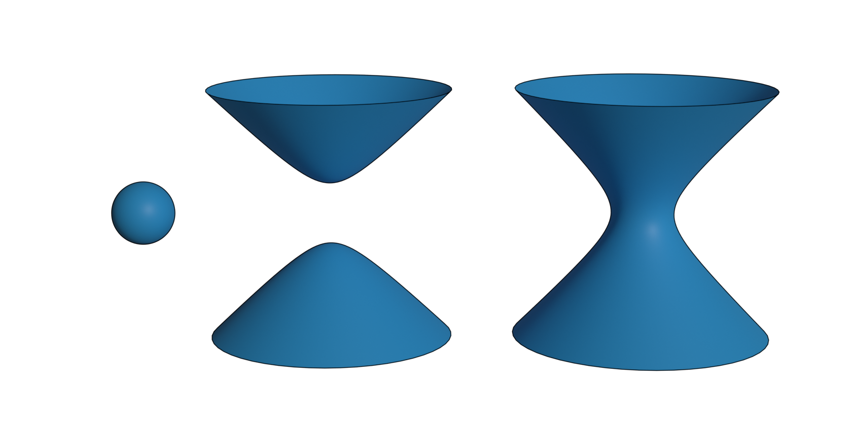
A quadric converted to a SmoothNet can further be converted to a DiscreteNet and then visualized in Blender. For more information on the sampling of nets (used in the conversion to a discrete net) see here.

>>> sphere = ddg.geometry.quadrics.Quadric(np.diag([1,1,1,-1]))
>>> sphere = ddg.to_blender_object_helper(sphere, sampling=[.1, 20, 'c'], name='sphere')

>>> one_sheeted_hyperboloid= ddg.geometry.quadrics.Quadric(np.diag([1,1,-1,-1]))
>>> one_sheeted_hyperboloid = ddg.to_blender_object_helper(one_sheeted_hyperboloid, sampling=[.1, 20, 'c'],
...                                                 name='one_sheeted_hyperboloid',location=[16,0,0], bounding_box=[5,5,4])

>>> two_sheeted_hyperboloid = ddg.geometry.quadrics.Quadric(np.diag([1,1,-1,1]))
>>> two_sheeted_hyperboloid = ddg.to_blender_object_helper(two_sheeted_hyperboloid, sampling=[.1, 20, 'c'],
...                                                 name='two_sheeted_hyperboloid', location=[6,0,0], bounding_box=[5,5,4])

Visualizing spheres

A two-dimensional sphere in three-dimensional space can be converted to a SmoothNet using the function to_smooth_net().

>>> sphere = ddg.geometry.spheres.Sphere(np.array([3.0, 0.0, 1.0, 1.0]), 1.0)
>>> sphere_net = ddg.to_smooth_net(sphere)

>>> print(type(sphere_net))
<class 'ddg.datastructures.nets.net.SmoothNet'>

The resulting smooth net can be directly visualized in Blender using to_blender_object(). For more details, see Nets.

Similarly we can convert a circle in any ambient dimension to a SmoothCurve using to_smooth_net().

A render of Ford circles using smooth nets.

>>> P1 = np.array([12.0, 0.0, 1.0, 1.0])
>>> P2 = np.array([0.0, 9.0, 1.0, 1.0])
>>> P3 = np.array([1.0, 5.0, 4.0, 7.0])
>>> center = P1 - P3
>>> circle = ddg.geometry.spheres.Sphere(center, 1.0, subspace=[P1, P2, P3])
>>> circle_net = ddg.to_smooth_net(circle)

>>> print(type(circle_net))
<class 'ddg.datastructures.nets.net.SmoothCurve'>

Note

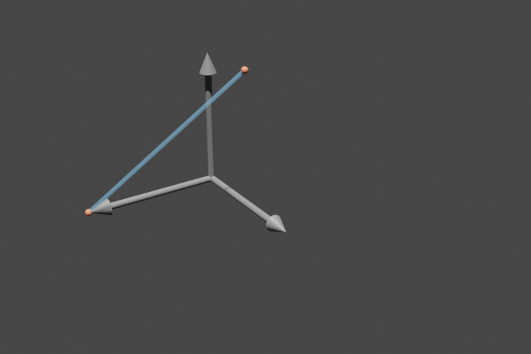
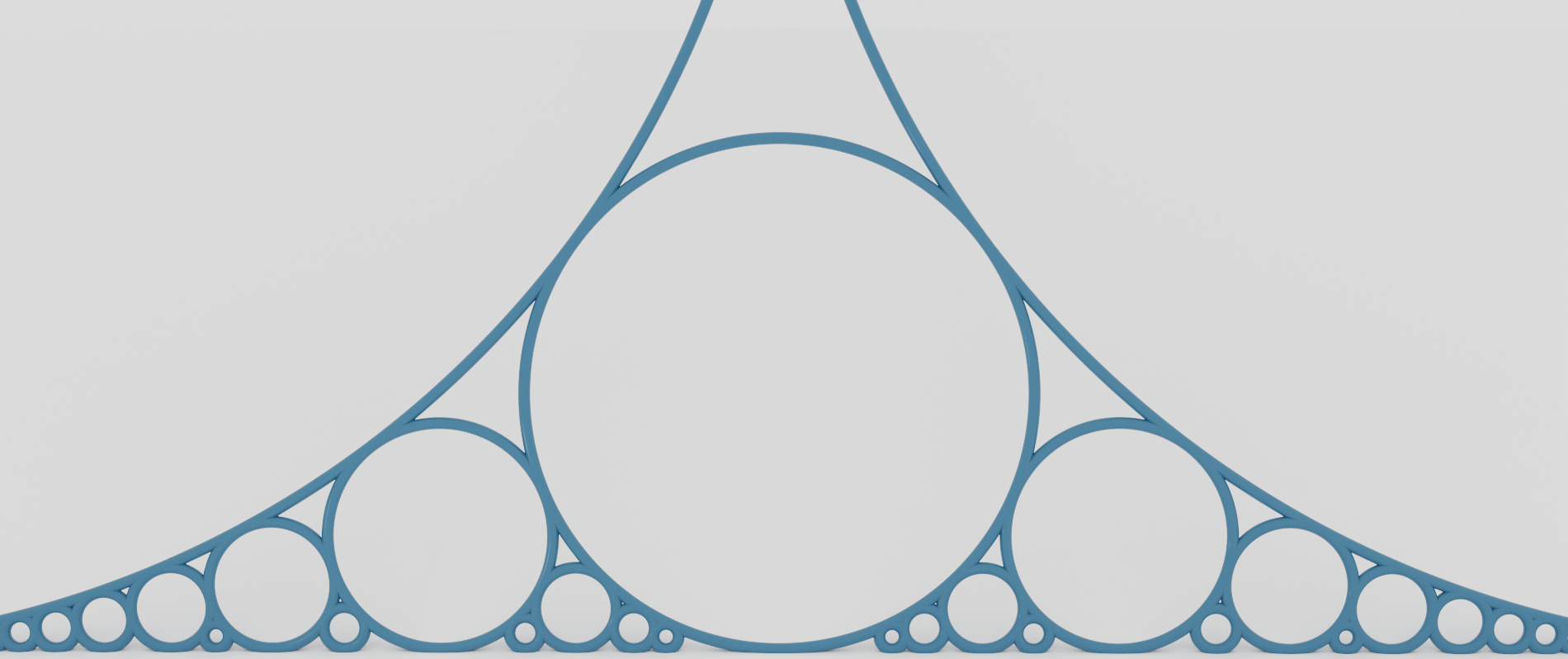
The smooth net of a circle in \(n\)-dimensional space depends on its radius, center and (optionally) its subspace.

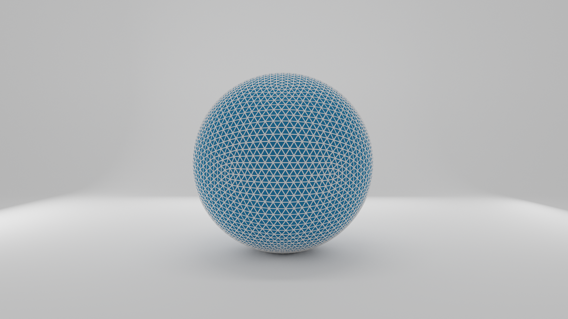
Another possible way to visualize a two-dimensional sphere is to convert it to an icosphere, which is a half-edge surface. This can be done using the function to_halfedge(). The icosphere can then be visualized in Blender using to_blender_object(). For more details, see The half-edge data structure.

A wireframe render of an icosphere.

Creating linked duplicate Blender objects

One can reuse the data (eg. mesh, bmesh, light, camera, etc.) of an existing Blender object in other new Blender objects using the function create_duplicate_linked(). In the most common use case, this data is a mesh. The resulting Blender objects then share the same mesh, which can be modified (for exemple in edit mode) to affect all the objects simultaneously. In order to place the newly created objects in space, a list of 4x4 matrices reprensenting the transformations from the original object must be passed.

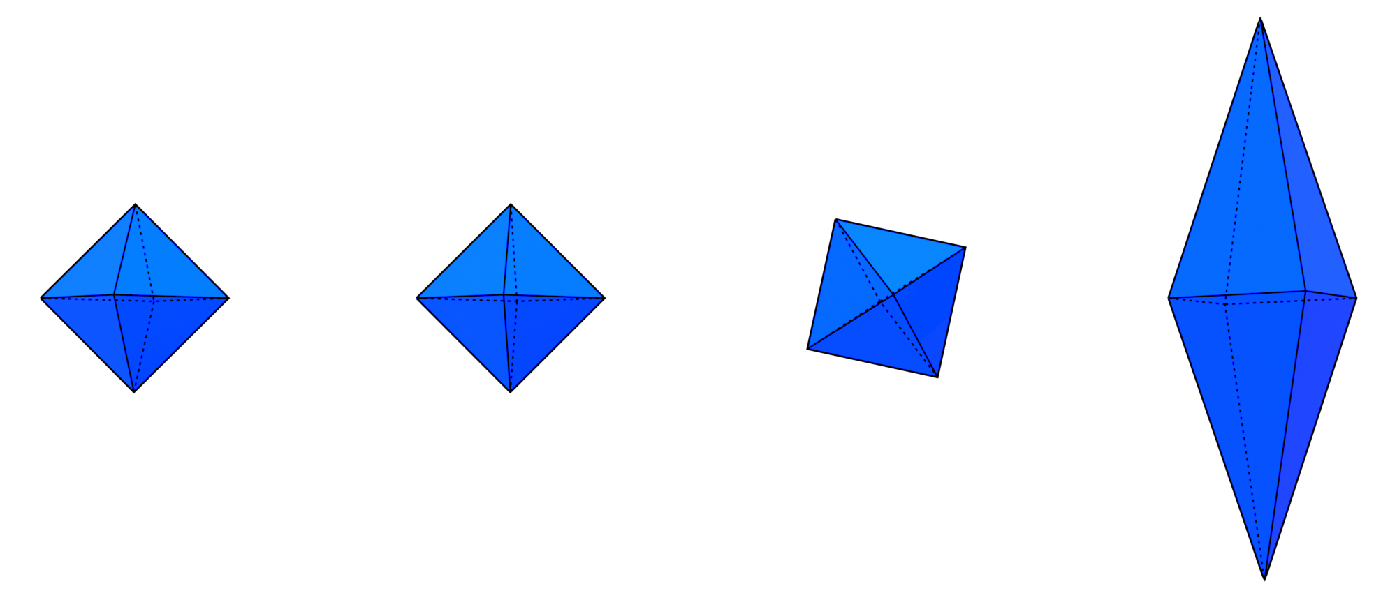
In this example we create 3 linked duplicates of an octahedron. The first is just translated, the second is rotated and the last is scaled.

>>> import ddg
>>> import numpy as np
>>> import ddg.datastructures.halfedge.surface_generator as gen
>>> from ddg.visualization.blender.object import create_duplicate_linked
>>> from ddg.visualization.blender import matrix 
>>> obj = gen.octahedron() 
>>> bobj = ddg.to_blender_object_helper(obj) 
>>> xTranslation = np.array([[1, 0, 0, 4],
...                         [0, 1, 0, 0],
...                         [0, 0, 1, 0],
...                         [0, 0, 0, 1]])
>>> rotation = matrix.rotation_angle_axis((0,1,0)) 
>>> scaling = np.array([[1, 0, 0, 0],
...                    [0, 2, 0, 0],
...                    [0, 0, 3, 0],
...                    [0, 0, 0, 1]]) 
>>> matrices = [xTranslation,
...            xTranslation @ xTranslation @ rotation,
...            xTranslation @ xTranslation @ xTranslation @ scaling] 
>>> duplicates = create_duplicate_linked(bobj, matrices) 

In the most common use case, this data is a mesh. The resulting Blender objects then share the same mesh, which can be modified (for exemple in edit mode) to affect all the objects simultaneously. In order to place the newly created objects in space, a list of 4x4 matrices reprensenting the transformations from the original object must be passed.

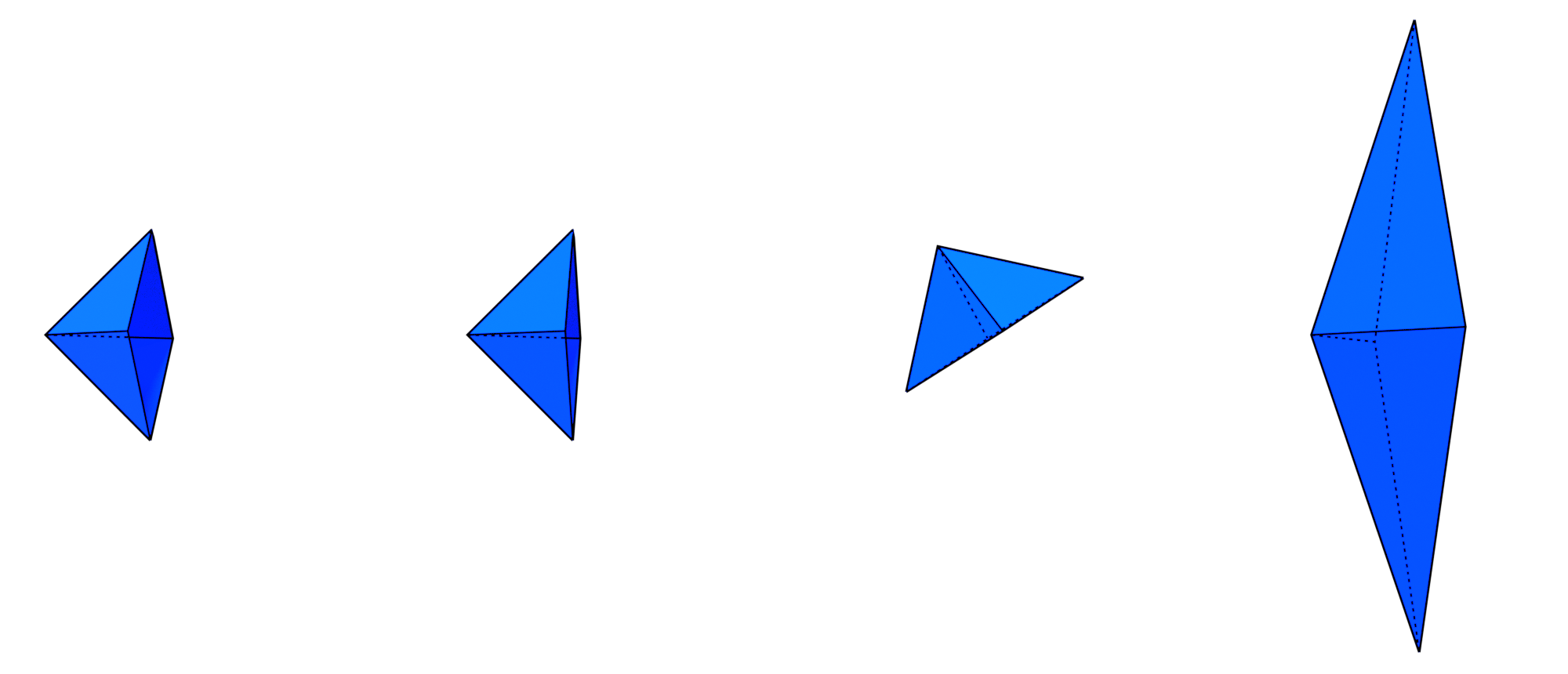
The result can be seen here :

We can then modify the mesh (here we removed a vertex):