Quadrics

Quadrics are hypersurfaces given by one quadratic homogeneous equation, for example ellipses, hyperbolas and ellipsoids. They are given by a symmetric matrix and are represented in our library by instances of the Quadric class.

Basic example

>>> import ddg
>>> import numpy as np
>>> quadric = ddg.geometry.quadrics.Quadric(np.diag([1.0, 1.0, 1.0, -1.0]))
>>> quadric
Quadric(
  array([[ 1.,  0.,  0.,  0.],
         [ 0.,  1.,  0.,  0.],
         [ 0.,  0.,  1.,  0.],
         [ 0.,  0.,  0., -1.]])
)

>>> np.array([1, 0, 0, 1]) in quadric
True

>>> quadric.rank
4

>>> quadric.corank
0

>>> print(quadric)
quadric in 3D projective space
signature: (3, 1)
matrix:
  [[ 1.  0.  0.  0.]
   [ 0.  1.  0.  0.]
   [ 0.  0.  1.  0.]
   [ 0.  0.  0. -1.]]

Quadrics induce an inner product:

>>> quadric = ddg.geometry.quadrics.Quadric(np.diag([1, 1, 1, -1]))
>>> quadric.inner_product(np.array([1, 1, 0, 1]), np.array([0, 1, 1, 0]))
1.0

Quadrics contained in subspaces

All quadrics have a containing subspace, similarly to spheres. By default, it is the whole space with the standard basis. This is important because of what the matrix represents: It is the gram matrix of the quadratic form with respect to the given basis of this subspace.

We can give the subspace as a Subspace object or as a list of points in homogeneous coordinates:

>>> conic_in_subspace = ddg.geometry.quadrics.Quadric(
...     np.diag([1.0, 1.0, -1.0]),
...     subspace=[[1, 1, 0, 1], [1, 0, 1, 1], [0, 0, 0, 1]],
... )
>>> print(conic_in_subspace)
conic contained in 2D subspace in 3D projective space
signature: (2, 1)
matrix:
  [[ 1.  0.  0.]
   [ 0.  1.  0.]
   [ 0.  0. -1.]]
basis of containing subspace (columns):
  [[1. 1. 0.]
   [1. 0. 0.]
   [0. 1. 0.]
   [1. 1. 1.]]

>>> p1, p2, p3 = conic_in_subspace.subspace.points
>>> conic_in_subspace.inner_product(p3, p3).round(decimals=10)
-1.0
>>> conic_in_subspace.inner_product(p1, p2).round(decimals=15) == 0.0
True
>>> (p1 - p3) in conic_in_subspace
True

Transforming the quadric actually transforms the subspace:

>>> F = np.diag([2, 2, 1, 1])
>>> conic_in_subspace = conic_in_subspace.transform(F)
>>> print(conic_in_subspace.matrix)
[[ 1.  0.  0.]
 [ 0.  1.  0.]
 [ 0.  0. -1.]]
>>> print(conic_in_subspace.subspace.matrix)
[[2. 2. 0.]
 [2. 0. 0.]
 [0. 1. 0.]
 [1. 1. 1.]]

Signatures

Quadrics have a signature method that optionally accepts the keyword arguments subspace (default None, i.e. the whole subspace) and affine (default False). The former can be used to get the signature of the quadratic form restricted to a subspace. The latter controls whether to return the usual signature of quadratic forms (which determines a quadric up to projective transformation) or an affine signature (which determines a quadric up to affine transformation). They are instances of the classes Signature and AffineSignature, which can be compared easily and much more:

>>> sgn = quadric.signature()
>>> print(sgn)
(3, 1)
>>> sgn == ddg.math.symmetric_matrices.Signature(1, 3)
True
>>> print(sgn.matrix)
[[ 1  0  0  0]
 [ 0  1  0  0]
 [ 0  0  1  0]
 [ 0  0  0 -1]]
>>> sgn.is_degenerate
False
>>> sgn.is_positive_definite
False
>>> sgn.is_negative_semi_definite
False
>>> sgn.is_indefinite
True
>>> sgn = quadric.signature(affine=True)
>>> print(sgn)
(3, 1)
last entry: -1
>>> sgn2 = ddg.math.symmetric_matrices.AffineSignature(3, 1, last_entry=1)
>>> print(sgn2.matrix)
[[ 1  0  0  0]
 [ 0  1  0  0]
 [ 0  0 -1  0]
 [ 0  0  0  1]]
>>> sgn == sgn2
False

An outlier are so-called parabolic signatures, which corresponds to matrices that cannot be diagonalized with an affine transformation:

>>> sgn = ddg.math.symmetric_matrices.AffineSignature(3, 1, last_entry="parabolic")
>>> print(sgn.matrix)
[[1 0 0 0]
 [0 1 0 0]
 [0 0 0 1]
 [0 0 1 0]]

Note that the two zeros on the diagonal correspond to a 1 and a -1 in the actual (projective) signature.

Polarization

We can polarize subspaces and quadrics using the polarize() method:

>>> quadric = ddg.geometry.quadrics.Quadric(np.diag([1, 1, 1, -2]))
>>> subspace = ddg.geometry.subspaces.Subspace([1, 0, 1, 2]).dualize()

>>> polar_space = quadric.polarize(subspace)
>>> polar_space
Point(array([...]))

>>> for p in subspace.points:
...     print(quadric.conjugate(p, polar_space.point))
...
True
True
True

The touching cone

We can also obtain the touching cone to a quadric of a point not lying on it using the utility function touching_cone():

>>> quadric_matrix = np.array(
...     [[1, 0, 0, 0], [0, 1, 0, 0], [0, 0, 0, 1], [0, 0, 1, 0]]
... )
>>> quadric = ddg.geometry.quadrics.Quadric(quadric_matrix)

>>> print(quadric.signature())
(3, 1)

>>> point = np.array([2, 0.5, 3, 2])
>>> point in quadric
False

>>> cone = ddg.geometry.quadrics.touching_cone(point, quadric)
>>> cone
Quadric(
  array([[-12.25,   1.  ,   4.  ,   6.  ],
         [  1.  , -16.  ,   1.  ,   1.5 ],
         [  4.  ,   1.  ,   4.  , -10.25],
         [  6.  ,   1.5 , -10.25,   9.  ]])
)

>>> print(cone.signature())
(1, 2, 1)

>>> cone.singular_subspace
Point(array([...]))

Note that the behavior of this function for quadrics contained in proper subspaces depends on a boolean keyword argument in_subspace. If it is True, the point must be contained in quadric.subspace and the subspace is treated as the ambient space. If it is False, the function looks at tangency in the whole ambient space. In the latter case, it can happen that the touching cone would be a solid cone, which we can not represent. In this case, we raise an Exception.

>>> Q = ddg.geometry.quadrics.Quadric(
...     np.diag([2, 1, -3]), subspace=[[1, 0, 0, 0], [0, 0, 1, 0], [0, 0, 0, 1]]
... )

>>> P_not_in_subspace = [0, 2.5, 0, 1]
>>> tc1 = ddg.geometry.quadrics.touching_cone(P_not_in_subspace, Q)
>>> print(tc1)
quadric in 3D projective space
signature: (2, 1, 1)
matrix:
  [[ 2.  0.  0.  0.]
   [ 0.  1.  0.  0.]
   [ 0.  0. -3.  0.]
   [ 0.  0.  0.  0.]]
basis of ambient space (columns):
  [[1.  0.  0.  0. ]
   [0.  0.  0.  2.5]
   [0.  1.  0.  0. ]
   [0.  0.  1.  1. ]]

>>> P_in_subspace = [2.5, 0, 0, 1]
>>> tc2 = ddg.geometry.quadrics.touching_cone(P_in_subspace, Q, in_subspace=True)
>>> print(tc2)
conic contained in 2D subspace in 3D projective space
signature: (1, 1, 1)
matrix:
  [[  6.    0.  -15. ]
   [  0.   -9.5   0. ]
   [-15.    0.   37.5]]
basis of containing subspace (columns):
  [[1. 0. 0.]
   [0. 0. 0.]
   [0. 1. 0.]
   [0. 0. 1.]]

>>> tc3 = ddg.geometry.quadrics.touching_cone(P_in_subspace, Q)
Traceback (most recent call last):
...
NotImplementedError: The join is a 'solid' cone, which we can't represent. Use touching_cone with in_subspace=True to obtain its boundary.

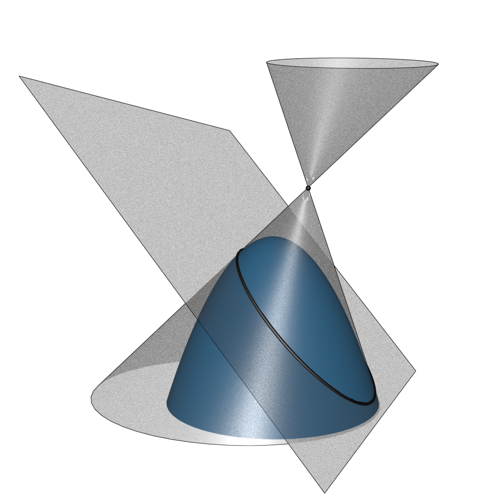
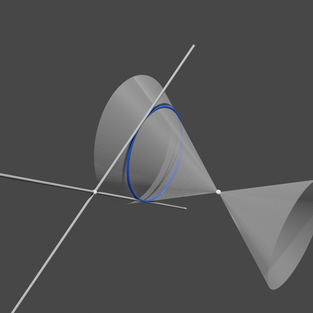
In this image you can see a conic contained in a subspace in blue, two points and some options for touching cones you can get:

Converting a quadric to a net

You can choose between a parametrization in affine or homogeneous coordinates by passing a parameter affine to to_smooth_net with the default being affine coordinates, since those are what’s needed for visualization.

>>> quadric = ddg.geometry.quadrics.Quadric(np.diag([1, 1, -1, -1]))

>>> quadric_net = ddg.to_smooth_net(quadric)
>>> len(quadric_net(0, 0))
3
>>> quadric_net = ddg.to_smooth_net(quadric, affine=False)
>>> len(quadric_net(0, 0))
4

Conversion to nets is supported for any conic or quadric contained in a line, plane or 3D subspace in any ambient space. If additionally the ambient dimension is 3, it can then be visualized in Blender:

Visualization in Blender

A guide on how to visualize quadrics in Blender can be found here: Visualizing quadrics.