Subspaces
The ddg.geometry.subspaces module contains classes and functions related to projective subspaces, i.e. points, lines, planes etc. These are instances of Subspace or Point.
Creating subspaces
The Subspace class is initialized with homogeneous coordinates:
>>> import ddg

>>> subspace = ddg.geometry.subspaces.Subspace([1, 0, 1, 0], [0, 1, 1, 1])
>>> subspace
Subspace(array([1., 0., 1., 0.]), array([0., 1., 1., 1.]))
>>> print(subspace)
Line in 3D projective space
Homogeneous coordinates (columns):
  [[1. 0.]
   [0. 1.]
   [1. 1.]
   [0. 1.]]
>>> subspace.dimension
1
>>> subspace.ambient_dimension
3
>>> subspace.at_infinity()
False
To get the points in affine coordinates, use the methods Subspace.affine_points() and Subspace.affine_matrix().
Note that we have passed the points as separate arguments. To create a subspace
using the columns or rows of a matrix as points, we have the utility functions
subspace_from_columns() and
subspace_from_rows():
>>> import numpy as np

>>> points = np.array([[1, 0], [0, 1], [1, 1], [0, 1]])
>>> subspace = ddg.geometry.subspaces.subspace_from_columns(points)
>>> subspace
Subspace(array([1., 0., 1., 0.]), array([0., 1., 1., 1.]))
There is also subspace_from_affine_points():
>>> x_axis = ddg.geometry.subspaces.subspace_from_affine_points([0, 0, 0], [1, 0, 0])
>>> print(x_axis)
Line in 3D projective space
Homogeneous coordinates (columns):
  [[0. 1.]
   [0. 0.]
   [0. 0.]
   [1. 1.]]
There is a special subclass Point
that subspaces with a single point automatically get cast to:
>>> p = ddg.geometry.subspaces.Subspace([1, 0, 1, 0])
>>> p
Point(array([1., 0., 1., 0.]))
>>> print(p)
Point in 3D projective space
Homogeneous coordinates: [1. 0. 1. 0.]
>>> p.point
array([1., 0., 1., 0.])
>>> p.at_infinity()
True
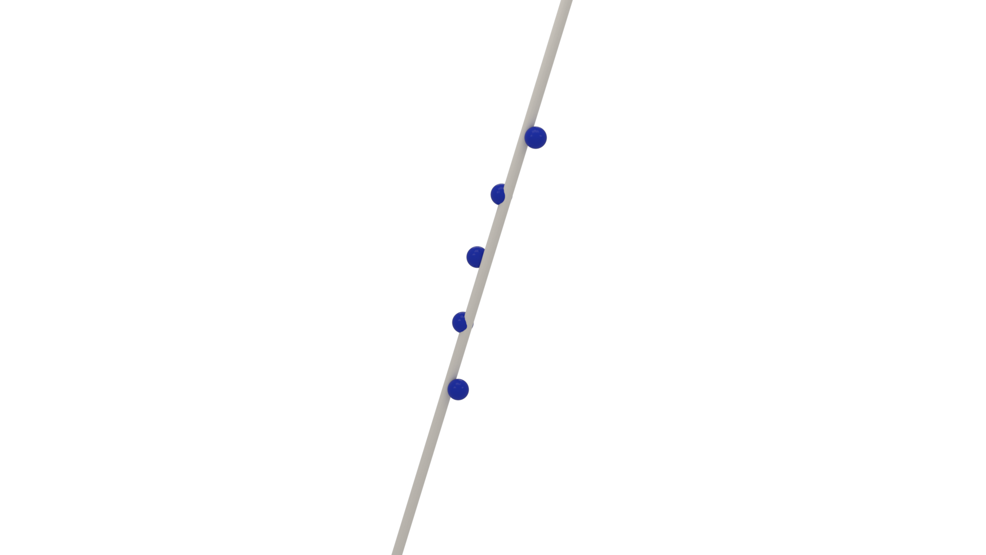
It is also possible to create a \(k\)-dimensional least-square subspace using least_square_subspace_from_affine_points() given the affine coordinates of \(N\) points.
>>> affine_coordinates = [
... np.array([-5.2, 3.1, 3.0, 4.6]),
... np.array([1.2, 0.2, 5.0, 1.0]),
... np.array([1.56, 0.9, 2.1, 0.43]),
... np.array([6.4, 4.0, 6.0, 0.0]),
... ]
>>> line = ddg.geometry.subspaces.least_square_subspace_from_affine_points(
... affine_coordinates, k=1
... )
>>> print(line)
Line in 4D projective space
Homogeneous coordinates (columns):
[[ 0.99 0.90091871]
[ 2.05 0.0336353 ]
[ 4.025 0.22091693]
[ 1.5075 -0.37203476]
[ 1. 0. ]]
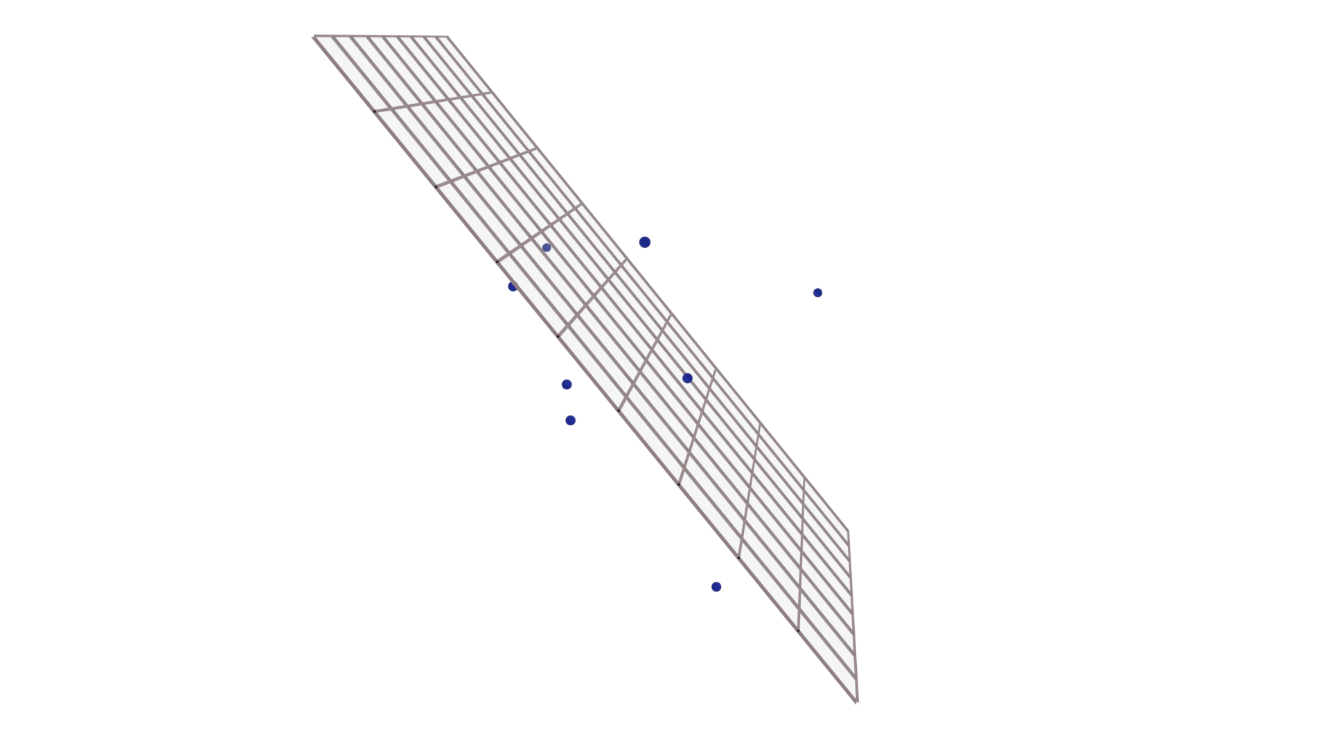
>>> plane = ddg.geometry.subspaces.least_square_subspace_from_affine_points(
... affine_coordinates, k=2
... )
>>> print(plane)
Plane in 4D projective space
Homogeneous coordinates (columns):
[[ 0.99 0.90091871 -0.01438605]
[ 2.05 0.0336353 -0.827788 ]
[ 4.025 0.22091693 -0.4272281 ]
[ 1.5075 -0.37203476 -0.36336788]
[ 1. 0. 0. ]]
Note that passing k=-1 returns a least-square hyperplane, i.e a subspace of dimension one less than ambient dimension.
>>> hyperplane = ddg.geometry.subspaces.least_square_subspace_from_affine_points(
...     affine_coordinates, k=-1
... )
>>> print(hyperplane)
Hyperplane in 4D projective space
Homogeneous coordinates (columns):
  [[ 0.99        0.90091871 -0.01438605  0.15173223]
   [ 2.05        0.0336353  -0.827788    0.4826233 ]
   [ 4.025       0.22091693 -0.4272281  -0.85701824]
   [ 1.5075     -0.37203476 -0.36336788 -0.09783564]
   [ 1.          0.          0.          0.        ]]
>>> hyperplane.dimension
3
>>> hyperplane.ambient_dimension
4
We can also pass a list of points as Point directly to the function least_square_subspace() where their affine coordinates are automatically used to get a \(k\)-dimensional least-square subspace.
>>> from ddg.geometry.subspaces import Point
>>> points = [
...     Point(np.array([1.0, 2.0, 1.0, 1.0])),
...     Point(np.array([0.0, 0.0, 1.0, 1.0])),
...     Point(np.array([2.0, 3.0, 3.0, 1.0])),
...     Point(np.array([5.0, 7.0, 1.0, 1.0])),
...     Point(np.array([6.0, 8.1, 0.0, 1.0])),
... ]
>>> plane = ddg.geometry.subspaces.least_square_subspace(points, 2)
>>> print(plane)
Plane in 3D projective space
Homogeneous coordinates (columns):
  [[ 2.8         0.59954182 -0.03854255]
   [ 4.02        0.79259899 -0.11002335]
   [ 1.2        -0.1110696  -0.99318142]
   [ 1.          0.          0.        ]]
>>> plane.dimension
2
>>> plane.ambient_dimension
3
Finally, we can use whole_space() to get the entire projective space of a specific dimension.
>>> whole_three_space = ddg.geometry.subspaces.whole_space(3)
>>> print(whole_three_space)
Whole space in 3D projective space
Homogeneous coordinates (columns):
  [[1. 0. 0. 0.]
   [0. 1. 0. 0.]
   [0. 0. 1. 0.]
   [0. 0. 0. 1.]]
Intersecting and joining
We can intersect and join subspaces with the functions ddg.geometry.intersection.meet and ddg.geometry.intersection.join. The join is similar to the sum of vector spaces.
>>> from ddg.geometry.subspaces import subspace_from_affine_points as sfap
>>> line = sfap([0, 1, -1], [1, 0, 0])
>>> point = sfap([0, 0, 1.5])
>>> plane = sfap([1, 0, 0], [2, 1, 0], [1, 0, 1])
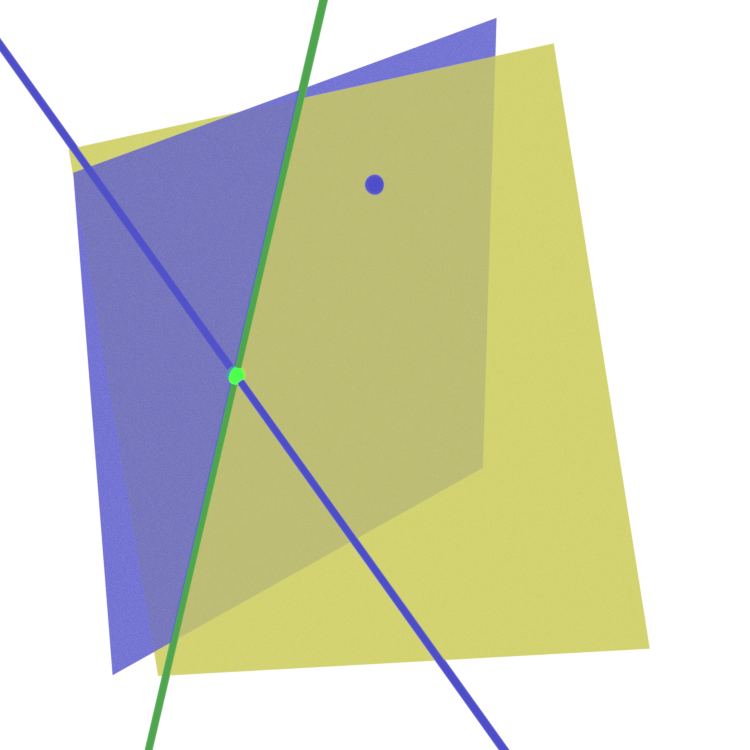
>>> join_plane = ddg.geometry.intersection.join(line, point)
>>> meet_line = ddg.geometry.intersection.meet(join_plane, plane)
>>> meet_point = ddg.geometry.intersection.meet(line, meet_line)
We can see all of these subspaces in the image below. The explicitly created objects are shown in blue, the join of the line and the point in yellow. The intersection of the plane and the line is shown in light green and the intersection of the plane and the join in dark green.
Dualization
To every k-dimensional subspace in n-dimensional projective space corresponds an (n-k-1)-dimensional dual subspace. In the simplest case, it essentially arises from taking the orthogonal complement of the subspace basis as the basis for the dual subspace.
>>> p_dual = p.dualize()
>>> p.dimension
0
>>> p_dual.dimension
2
Bisectors
The subspaces module provides functions for
creating bisections.
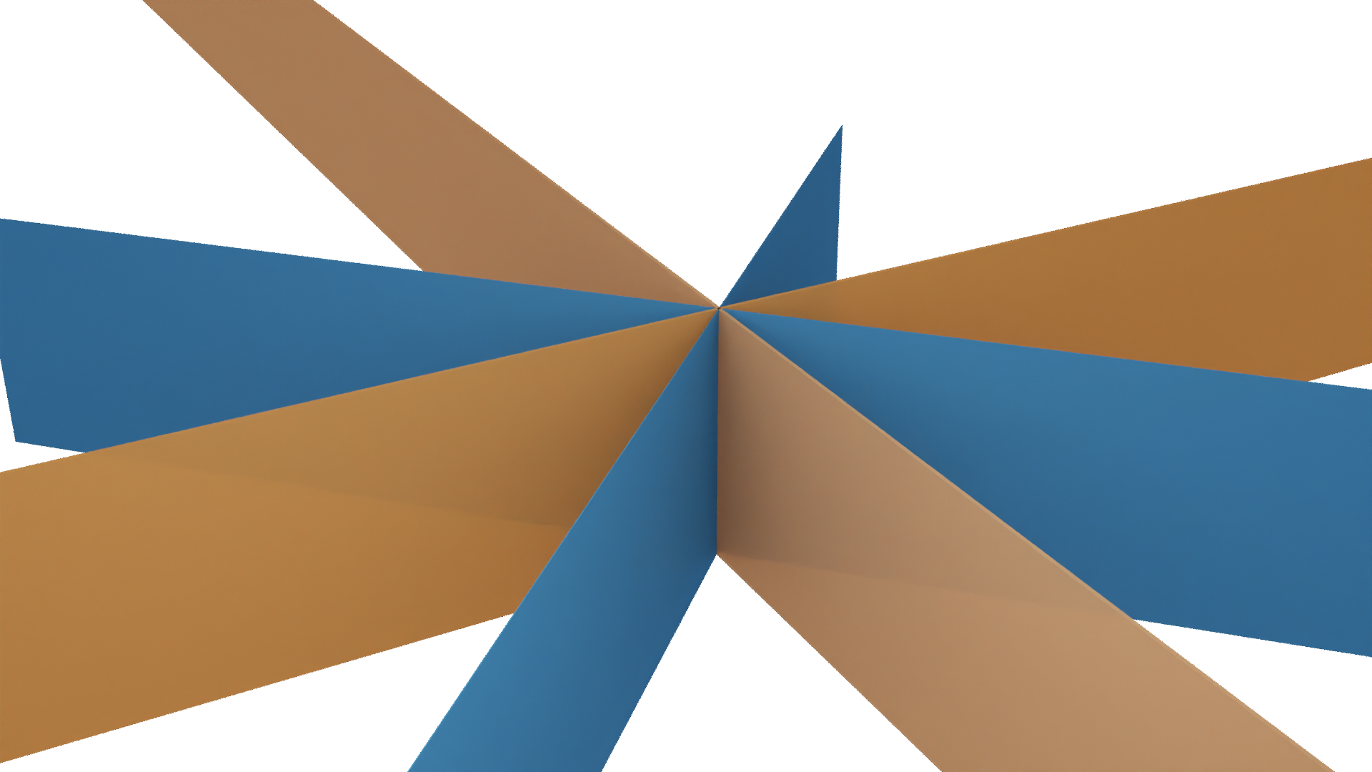
It provides angle_bisectors()
which, given two hyperplanes, computes the two angle bisecting hyperplanes.
Alternatively one can also use
angle_bisector_orientation_preserving() or
angle_bisector_orientation_reversing()
for a specific one of the two bisectors.
>>> from ddg.geometry.subspaces import hyperplane_from_normal, normal
>>> from ddg.geometry.subspaces import angle_bisectors
>>> h1 = hyperplane_from_normal((1, 0, 0), level=0)
>>> h2 = hyperplane_from_normal((0, 1, 0), level=0)
>>> h_preserving, h_reversing = angle_bisectors(h1, h2)
>>> normal(h_preserving)
array([ 0.70710678,  0.70710678, -0.        ])
>>> normal(h_reversing)
array([ 0.70710678, -0.70710678,  0.        ])
This will result in the following image.
Similarly, you can use perpendicular_bisector()
to obtain an orthogonal hyperplane intersecting the join of two points
in their (affine) midpoint.
>>> from ddg.geometry.subspaces import subspace_from_affine_points, normal, Point
>>> from ddg.geometry.subspaces import perpendicular_bisector
>>> p1 = Point((0, 0, 1))
>>> p2 = Point((1, 1, 1))
>>> orthogonal_line = perpendicular_bisector(p1, p2)
>>> normal(orthogonal_line)
array([-0.70710678, -0.70710678])
Which will result in the following image.

This works for arbitrary dimensions.
>>> from ddg.geometry.subspaces import subspace_from_affine_points, normal, Point
>>> from ddg.geometry.subspaces import perpendicular_bisector
>>> p1 = Point((0, 0, 0, 1))
>>> p2 = Point((1, 1, 1, 1))
>>> orthogonal_hyperplane = perpendicular_bisector(p1, p2)
>>> orthogonal_hyperplane.affine_points
[array([-2.1941919 ,  4.36085856, -0.66666667]), array([-2.1941919 , -0.66666667,  4.36085856]), array([0.93303028, 0.28348486, 0.28348486])]
>>> normal(orthogonal_hyperplane)
array([0.57735027, 0.57735027, 0.57735027])
Converting subspaces to nets
Subspaces of any dimension can simply be converted to nets using ddg.conversion.nets.core.to_smooth_net(), accessible directly as ddg.to_smooth_net. There are two different parametrizations available using the boolean keyword argument convex. You can also choose whether the net should output homogeneous or affine coordinates using the keyword affine. Both are True by default since that yields a net of the kind needed for visualization.
The “convex” parametrization
The convex=True parametrization is the one used for visualization. It only works for subspaces not at infinity and depends on the given basis of the subspace, i.e. subspace.points, which we will write as \((u_0,\dots,u_k)\). We denote by \(\tilde{u}_i\) the \(i\)-th basis vector dehomogenized, i.e. with last component normalized to either 0 or 1. First, we take a look at the two most important special cases:
The first is where all basis vectors \(u_0,\dots,u_k\) are points not at infinity. the parametrization is
\[[\tilde{u}_0 + \lambda_1 (\tilde{u}_1 - \tilde{u}_0) + \dots + \lambda_k (\tilde{u}_k - \tilde{u}_0)],\]so in particular \((0,\dots,0) \mapsto [u_0]\) and \(e_j \mapsto [u_j]\). This form is useful for drawing line segments for example: Say you are converting
Subspace(u0, u1)to a curve. Simply restrict the domain of the curve to[0, 1]and you will get the line segment between \([u_0]\) and \([u_1]\) (See Restricting the domain).In the 2D case, this will produce a parallelogram.
The other special case is where one basis vector (assume \(u_0\)) is a point not at infinity and all others are at infinity. In this case, the parametrization is
\[[\tilde{u}_0 + \lambda_1 u_1 + \dots + \lambda_k u_k].\]This case is useful for getting parametrizations that are centered around a certain point. For example, if the \(u_1,\dots,u_k\) are orthonormal and you restrict the domain to
[[-1, 1],...,[-1, 1]], you will get a symmetric parametrization around \([u_0]\), for example a square or a cube.
Now the general case: Let \((u_{ij})\) be subspace.matrix, i. e. \(u_{ij}\) is the \(i\)-th entry of the basis vector \(u_j\). We assume that \(u_0\) is not at infinity. If it is, a vector not at infinity will be moved to the first position. Then the full formula is:
This parametrization always produces vectors with last entry equal to 1.
>>> subspace = ddg.geometry.subspaces.Subspace([0, 0, 1, 0]).dualize()
>>> print(subspace)
Plane in 3D projective space
Homogeneous coordinates (columns):
  [[ 0.  1. -0.]
   [ 1.  0. -0.]
   [ 0.  0. -0.]
   [ 0.  0. -1.]]

>>> plane_net = ddg.to_smooth_net(subspace)
>>> plane_net(0, 0)
array([0., 0., 0.])
>>> plane_net(1, 0)
array([0., 1., 0.])
>>> plane_net(0, 1)
array([1., 0., 0.])
There are a few utility functions and methods available that help with creating better “convex” parametrizations:
ddg.geometry.subspaces.orthonormalize_subspace()aliasSubspace.orthonormalize()Computes a completely new basis \((u_0,\dots,u_k)\) that produces a parametrization of the form \(u_0 + \lambda_1 u_1 + \dots + \lambda_k u_k\), where \(u_0\) is the point in the subspace closest to the origin and \(u_1,\dots,u_k\) are orthonormal direction vectors at infinity.
ddg.geometry.subspaces.center_subspace()aliasSubspace.center().This sets the center of the parametrization. Basically replaces \(u_0\) with any other desired point in the subspace.
ddg.geometry.subspaces.orthonormalize_and_center_subspace()aliasSubspace.orthonormalize_and_center().Sets the center of the parametrization and orthonormalizes the basis simultaneously.
The homogeneous parametrization
The convex=False parametrization takes k+1 parameters and simply returns a
linear combination of the given basis vectors.
>>> subspace = ddg.geometry.subspaces.Subspace([0, 0, 1, 0]).dualize()
>>> print(subspace)
Plane in 3D projective space
Homogeneous coordinates (columns):
  [[ 0.  1. -0.]
   [ 1.  0. -0.]
   [ 0.  0. -0.]
   [ 0.  0. -1.]]

>>> plane_net_homogeneous = ddg.to_smooth_net(subspace, affine=False, convex=False)
>>> plane_net_homogeneous(1, 0, 0)
array([0., 1., 0., 0.])
>>> plane_net_homogeneous(1, 1, 1)
array([ 1.,  1.,  0., -1.])
Restricting the domain
To restrict the domain, to_smooth_net has a keyword domain. It can take
either a domain object or its representation as a list of lists. See
Domains for more information.
>>> plane_net = ddg.to_smooth_net(subspace, convex=True, affine=True)
>>> plane_net.domain
SmoothRectangularDomain([[-inf, inf, False], [-inf, inf, False]])
>>> plane_net_restricted = ddg.to_smooth_net(
...     subspace, convex=True, affine=True, domain=[[0, 1], [0, 1]]
... )
>>> plane_net_restricted.domain
SmoothRectangularDomain([[0.0, 1.0, False], [0.0, 1.0, False]])
Visualization in Blender
A guide on how to visualize Subspaces in Blender can be found here: Visualizing Subspaces.