Möbius Pencil of Circles

In this tutorial, our aim is to visualize pencils of Möbius circles. This is explained below, expecting a bit of basic knowledge of geometry. If you are not that interested, or do not completely understand the mathematical background - that is okay too. You can still go on with the tutorial. The nice thing about visualization is, it helps us understand what is happening.

In the following, we explain how to create this python script: Möbius Pencil of Circles Script, and use it to visualize the objects in Blender.

Mathematical Background

What is a Möbius pencil of circles?

Möbius geometry in \(\widehat{\mathbb{R}^2} = \mathbb{R}^{2} \cup \{\infty\}\) corresponds to geometry on the unit sphere \(S^2\) via stereographic projection. Thus, circles in two-dimensional Möbius geometry correspond to circles on \(S^2\), which are intersections of \(S^2\) with planes. By polarity, a plane intersecting \(S^2\) corresponds to a point outside \(S^2\).

If we now consider a line in \(\mathbb{R}^3\), by polarity its points define a one-parameter family of planes in \(\mathbb{R}^3\) and therefore a one-parameter family of spherical circles, and hence - via stereographic projection - a so called Möbius pencil of circles in \(\widehat{\mathbb{R}^2}\).

The one-parameter family of planes all intersect in a common line, the polar line of the given line, which again represents a Möbius pencil of circles. In \(\widehat{\mathbb{R}^2}\) this polar pencil represents a family of circles where each circle intersects all circles in the first pencil orthogonally.

Setup

Start Blender from the terminal, so you can read error messages. More on how to start and setup Blender, you find here: Scripting in Blender.

In the Blender GUI, create a new script, add the following imports to your new script, and execute with “Alt”+”P”.

import numpy as np

import ddg
from ddg.blender.collection import collection
from ddg.blender.material import material

To start with a clean Blender file, we first remove all objects from the scene with clear().

ddg.blender.scene.clear(remove_collections=True)
ddg.blender.material.clear()

For more on the clear functions, see Clear Functions.

In this script, our aim is to generate a lot of Blender objects, and we want to be able to display them independently from one another. To achieve this, we will use Blender collections, enabling us to show/hide a lot of objects simultaneously. New collections can be created with the following command:

# for objects that were created for didactical purposes
example_coll = collection("example stuff")

# for objects belonging to the 3D moebius picture
mob_geo_coll = collection(
    "Moebius geometry",
    children=[
        ["lines", "points on line", "points on polar line"],
        "spherical circles",
        "polar spherical circles",
    ],
)

# for objects belonging to the 2D euclidean picture
euc_geo_coll = collection(
    "Euclidean geometry", children=["Euclidean circles", "orthogonal Euclidean circles"]
)

# for objects belonging to the light projection picture
projection_coll = collection("projection with light")

# for the slider function
slider_circles_coll = collection("slider circles")

You can pass a list of children to the function collection(). If an entry of the list is a string, it will create a child with corresponding name. If an entry of the list is a list of strings, the first string determines the name of the child collection, the others will create grandchildren, i.e children of the child’s collection. If the parent collection already exists, it returns that collection object, ignoring the children.

We are ready to create some objects.

Sphere and Line

Sphere

First, we want to create the sphere as a Quadric. Add the following to your script.

s2 = ddg.geometry.Quadric(np.diag([1, 1, 1, -1]))

A Quadric is created by its symmetric matrix. More information on Quadrics, you can find here.

To display the sphere in Blender, we have to convert it to a Blender object. This is easily done with the conversion function convert()!

bobj_s2 = ddg.blender.convert(s2, "s2", material="s2", collection=mob_geo_coll)
ddg.blender.mesh.shade_smooth(bobj_s2)

As for any smooth object, for the quadric to be displayed in Blender, it needs to be discretized using a sampling. The function convert() has a built-in sampling for quadrics which should produce a nice-looking result in most cases.

If you want more control over how the result is going to look, you will have to sample it yourself. For this, you will first need to convert the object to a SmoothNet. This can then, by a sampling, be converted to a DiscreteNet. For more information, have a look at the nets user’s guide. The sampling options are explained here.

The given name determines the name of the object in Blender.

Line

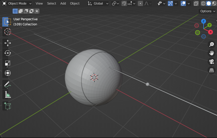
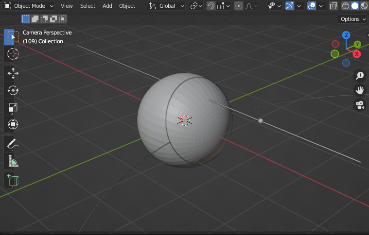
Next, we want to create and display a line. For that, we use Subspace, which is a class for projective subspaces. Here we give two examples one line that intersects the sphere and another line that is tangential to the sphere. With these two you can generate the configurations of the images at the top. So let’s choose

# line through S2
p1, p2 = np.array([-4, 0, 0.5, 1]), np.array([4, 0, 0.5, 1])
#
# p1, p2 = np.array([-1, 1, 0, 1]), np.array([1, 1, 0, 1])
l = ddg.geometry.Subspace(p1, p2)

A subspace can be simply defined by the vectors that span it. Note, that we want a line in 3D projective space, which corresponds to a 2D vector subspace of \(\mathbb{R}^4\). That’s why we have two 4D vectors. More on subspaces, you can find here.

Next, we create a SmoothNet out of the subspace, to obtain an affine image of the projective subspace, that is a line in 3D space. Before we do so, we orthonormalize and center the subspace.

# orthonormalize and center l
l = l.orthonormalize_and_center((p1 + p2) / 2)

# create smooth net
l_net = ddg.to_smooth_net(l, domain=[[-4, 4]], affine=True, convex=True)

The argument affine is given to obtain an affine image of the projective line. The convex=True argument means, that the net function of the resulting SmoothNet is the convex combination of the vectors spanning the subspace. By setting the domain of the SmoothNet to domain=[[-4,4]], we obtain a line segment symmetrical around the center of the line.

And finally, we convert it to a Blender object by:

# to blender
bobj_l = ddg.blender.convert(
    l,
    "line",
    collection=mob_geo_coll.children[0],
    material="line",
)
bobj_l.data.bevel_depth = 0.01

The given domain is interpreted as domain of the net function and determines the length of the line. We add the line to the collection we created. The last argument, given in this form of a dictionary, determines the thickness of the line. Feel free to play with it.

Spherical and Planar Circles

Next, we will see how a point on the line l corresponds to a circle on s2, and how the spheric circle corresponds to a planar circle.

Spherical Circles

For a given point, we want to calculate its polar plane with respect to s2, as well as the intersection of the plane with s2. These intersection should then be converted to blender objects, so that we can see them. And this gives us our spherical circles.

We choose a point on our line l. When given a point of its domain as an argument, a SmoothNet returns its value at this point:

# get a point
pt = l_net(2)

Now, we want to display the sampled point in Blender, as a little sphere. The sampled point is just an affine image of a point on l. We homogenize it,

# homogenize pt
pt_homogenized = ddg.math.projective.homogenize(pt)

and convert it to a Subspace.

# convert point to subspace
pt_projective = ddg.geometry.Subspace(pt_homogenized)

We give the radius for the size of the sphere that visualizes the point.

# display point in blender
bobj_pt = ddg.blender.vertices(
    pt_projective,
    "point",
    radius=0.05,
    material="point",
    collection=example_coll,
)

Now, we can make use of the methods for Subspaces and calculate the polar plane

# calculate its polar plane
plane = s2.polarize(pt_projective)

and calculate the intersection of it with the sphere.

# calculate intersection circle
circ_on_sphere = ddg.geometry.meet(plane, s2)

Trying to convert an empty intersection to a blender object yields an error, so first, we check if the intersection is empty by checking its dimension.

# check if intersection is not empty
if circ_on_sphere.dimension != -1:
    bobj_circ_on_sphere = ddg.blender.convert(
        circ_on_sphere,
        "spherical circle",
        collection=example_coll,
        material="spherical circle",
    )
    bobj_circ_on_sphere.data.bevel_depth = 0.005

This gives us:

Planar Circles

Next, we want to stereographically project the spherical circle onto the plane.

For this we create a plane to project on as a subspace and stereographically project the circle:

# stereographic project
euc_plane = ddg.geometry.subspace_from_affine_points_and_directions(
    [[0, 0, 0]], [[1, 0, 0], [0, 1, 0]]
)
circ_on_plane = ddg.geometry.stereographic_project(circ_on_sphere, euc_plane)

# convert to blender
bobj_circ_on_plane = ddg.blender.convert(
    circ_on_plane,
    "planar circle",
    collection=example_coll,
    material="planar circle",
)
bobj_circ_on_plane.data.bevel_depth = 0.005

bobj_euc_plane = ddg.blender.convert(
    euc_plane,
    "euc_plane",
    material="euc plane",
    collection=euc_geo_coll,
)

In general the function stereographic_project() takes the point to project from and the plane to project to as arguments. In our case the projection point, the north pole, is precisely the default argument of the function.

And we get:

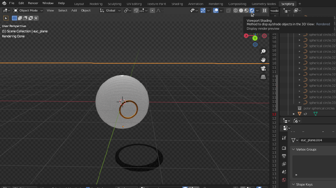
Alternatively: Shadows

We can also obtain the planar circles in a different way, putting a Blender light inside the sphere and looking at its shadow.

# stereographic project
light = ddg.blender.light.light(
    type_="POINT", location=[0, 0, 1], energy=600, collection=projection_coll
)
light.data.shadow_soft_size = 0

bobj_euc_plane.is_shadow_catcher = True

Here you may want to move the plane euc_plane a little bit lower so it does not intersect s2 so you can see the shadow of all circles. If you want to see the shadow in Blender you have to select the Rendered Viewport Shading.

Möbius Pencil of Circles

If we now consider the corresponding circles for all points on a line, that is called a Möbius pencil of circles. To visualize this pencil, we need to choose some points on the line, and then for each point proceed as above.

Circles Function for a Point

First, we write a function that takes a point and creates the corresponding spherical and planar circle. This function does the job:

def circles_from_point(
    pt,
    pt_name,
    circ_name,
    planar_name,
    pt_coll=None,
    spherical_coll=None,
    planar_coll=None,
    material_spherical=None,
    material_planar=None,
):
    """
    Create the point, the corresp. spherical circle,
    and the corresp. planar circle.

    Parameters
    ----------
    pt : array of length 3

    pt_coll,
    spherical_coll,
    planar_ coll : Blender Collections (default=None)

    material_spherical: string or bpy.tupes.Material
    material_planar: string or bpy.types.Material

    Returns
    -------
    None or list
    """

    # display point in blender
    bobj_pt = ddg.blender.vertices(
        ddg.nets.PointNet(pt),
        pt_name,
        radius=0.05,
        collection=pt_coll,
        material="point",
    )

    # homogenize pt
    pt_homogenized = ddg.math.projective.homogenize(pt)

    # convert point to subspace
    pt_homogenized = ddg.geometry.Subspace(pt_homogenized)

    # calculate its polar plane
    plane = s2.polarize(pt_homogenized)

    # calculate intersection circle
    circ_on_sphere = ddg.geometry.meet(plane, s2)

    # check if intersection is not empty
    if circ_on_sphere.dimension != -1:

        # convert spherical circle to blender
        bobj_circ_on_sphere = ddg.blender.convert(
            circ_on_sphere,
            circ_name,
            collection=spherical_coll,
            material=material_spherical,
        )
        bobj_circ_on_sphere.data.bevel_depth = 0.006

        # stereographic project
        circ_on_plane = ddg.geometry.stereographic_project(circ_on_sphere, euc_plane)

        # convert planar circle to blender
        bobj_circ_on_plane = ddg.blender.convert(
            circ_on_plane,
            planar_name,
            collection=planar_coll,
            material=material_planar,
        )
        bobj_circ_on_plane.data.bevel_depth = 0.006

        return [bobj_pt, bobj_circ_on_sphere, bobj_circ_on_plane]

    else:
        return [bobj_pt]

Wrapper Function for Points on a Line

Get the corresponding circles for a point on l by:

circles_from_point(
    l_net(1.3),
    "p1.3",
    "circ1.3",
    "plan1.3",
    pt_coll=mob_geo_coll.children[0].children[0],
    spherical_coll=mob_geo_coll.children[1],
    planar_coll=euc_geo_coll.children[0],
    material_spherical="spherical circle",
    material_planar="planar circle",
)

Adding a Slider for a Varying Point on Line

Next, we will add a slider to the blender GUI, with which we can regulate certain parameters in the creation of our objects. This is explained in more detail in this docs entry. In our case, we want to vary the parameter which determines the point on the line l.

The following code will add such a slider:

callback_collection = ddg.blender.collection.collection("callback")


def callback(t):
    ddg.blender.collection.clear([callback_collection], deep=True)
    circles_from_point(
        l_net(t),
        "p_slider",
        "circ_slider",
        "plan_slider",
        pt_coll=callback_collection,
        spherical_coll=callback_collection,
        planar_coll=callback_collection,
    )


ddg.blender.props.add_props_with_callback(callback, ("t",), 1.0)

To find the slider in the blender GUI, go to the viewport, press “N” to open the side menu, and go to the “DDG” tab. There it is.

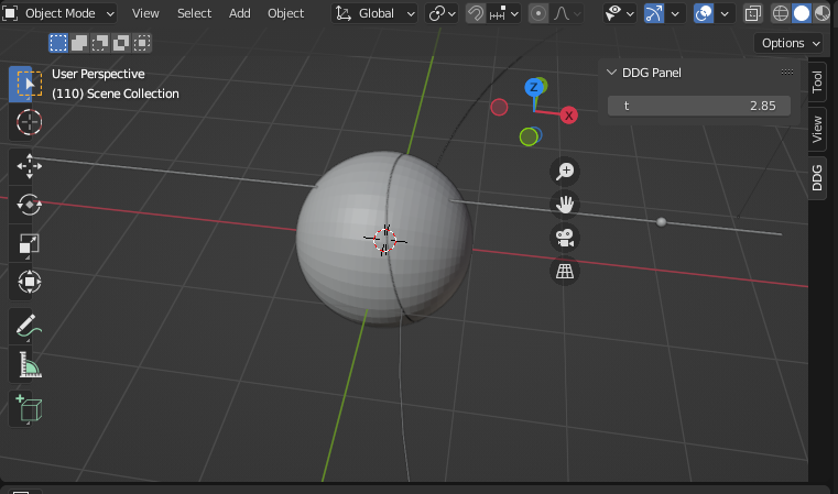
Change the parameter t, to see how the point and the circles change! But be careful sliders don’t work (well) with collections as they modify collections themselves. Its better not to work with collections when using sliders.

Visualize some Circles of the Pencil

To get a nice image of the pencil, we can sample points on the corresponding line, and then plot the circles for each of the points.

First, we need a sampling of the domain of the line. That is, a list with numbers. Let’s use linear sampling here (equidistant points). Of course you could try something else at home. It’s also fun to play with the number of samples.

# LINEAR SAMPLING OF DOMAIN
# this function takes arg3 samples equidistantly of the intervall [arg1,ag2]

sample = np.linspace(-3, 3, 30)

In the sampling, the first two arguments correspond to the domain of the lines, and the third is the number of samples.

Now, we can easily create some circles in the pencil:

# visualize pencil
for i, t in enumerate(sample):
    circles_from_point(
        l_net(t),
        f"p_{i}",
        f"circ_{i}",
        f"plane_{i}",
        pt_coll=mob_geo_coll.children[0].children[0],
        spherical_coll=mob_geo_coll.children[1],
        planar_coll=euc_geo_coll.children[0],
        material_spherical="spherical circle",
        material_planar="planar circle",
    )

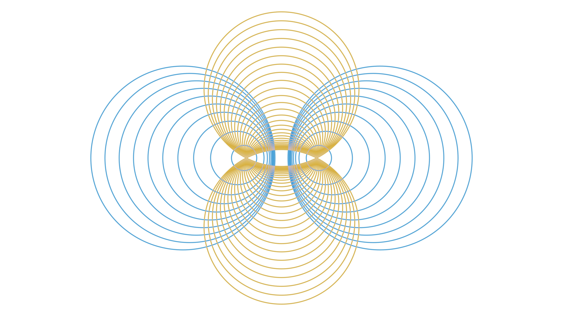
It is very useful, to pass collections here, so we can hide and show the different groups of objects as we wish. For example, hiding the collections with the points gives us:

Nice!

Orthogonal Pencil

Consider the Möbius pencil of circles for the polar line of l. All circles of this pencil intersect all circles in the pencil corresponding to l orthogonally.

With pyddg, we can easily polarize the Subspace l with respect to the Quadric s2 to obtain the polar line as a Subspace. We then proceed as before, to create the corresponding orthogonal pencil!

# get polar subspace of l
polar_l = s2.polarize(l)

# orthonormalize
polar_l = polar_l.orthonormalize()

# convert to net
polar_l_net = ddg.to_smooth_net(polar_l, domain=[[-4, 4]], affine=True, convex=True)

# convert to blender
bobj_polar = ddg.blender.convert(
    polar_l,
    "polar line",
    collection=mob_geo_coll.children[0],
)
bobj_polar.data.bevel_depth = 0.01

# visualize orthogonal pencil
for i, t in enumerate(sample):
    circles_from_point(
        polar_l_net(t),
        f"polar_p_{i}",
        f"polar_c_{i}",
        f"polar_plane_{i}",
        pt_coll=mob_geo_coll.children[0].children[1],
        spherical_coll=mob_geo_coll.children[2],
        planar_coll=euc_geo_coll.children[1],
        material_spherical="polar spherical circle",
        material_planar="polar planar circle",
    )

And we get:

Render an Image

Before we render an image, we need to add a camera and light to the Blender scene and create materials for our objects.

# add camera and light
cam = ddg.blender.camera.camera(location=(0, 0, 19))
light = ddg.blender.light.light(location=(0, 0, 50))

light.data.use_shadow = False

How to create such a setup and render an image is further explained here Camera and Light and here Rendering.

Materials can be created and assigned to objects in the blender GUI. If you have a lot of objects, it’s convenient to assign materials via script! Basic materials can also be created in the script, as explained here: Creating and Setting Materials.

We add the following materials in the beginning of our script, before object creation. (The names of the materials agree with the names of the materials we use in object creation).

material(name="s2", color=(0.413, 0.828, 0.990), specular=0.4, roughness=0.6, alpha=0.5)

material(name="euc plane", color=(0, 0, 0), specular=0.5, roughness=1, alpha=1)

material(
    name="polar spherical circle",
    color=(1, 0.533, 0.044),
    specular=0.1,
    roughness=1,
    alpha=1,
)

material(
    name="spherical circle", color=(0.029, 0.139, 1), specular=0.1, roughness=1, alpha=1
)

material(
    name="polar planar circle",
    color=(1, 0.533, 0.044),
    specular=0.1,
    roughness=0.9,
    alpha=1,
)

material(
    name="planar circle", color=(0.029, 0.139, 1), specular=1, roughness=1, alpha=1
)

You choose which collections (or objects) to hide and show for an image. In the python script, collections can be hidden with

example_coll.hide_render = True
example_coll.hide_viewport = True
projection_coll.hide_render = True
projection_coll.hide_viewport = True
slider_circles_coll.hide_render = True
slider_circles_coll.hide_viewport = True

Keep in mind that there are two parameters, hide_viewport and hide_render, that can be set. Here, we have hidden certain collections so that when executing the script, the resulting image is less cluttered.

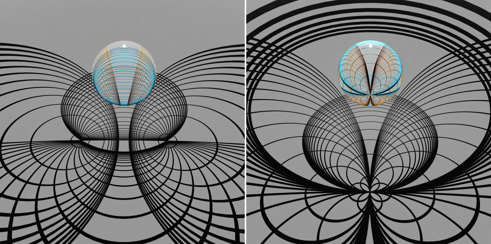
Now by hiding and showing different collections in the blend file we created, and playing with the materials, light and camera, we can then render beautiful images, like:

(Serving suggestion)