Envelopes and Orthogonal Trajectories of Families of Circles
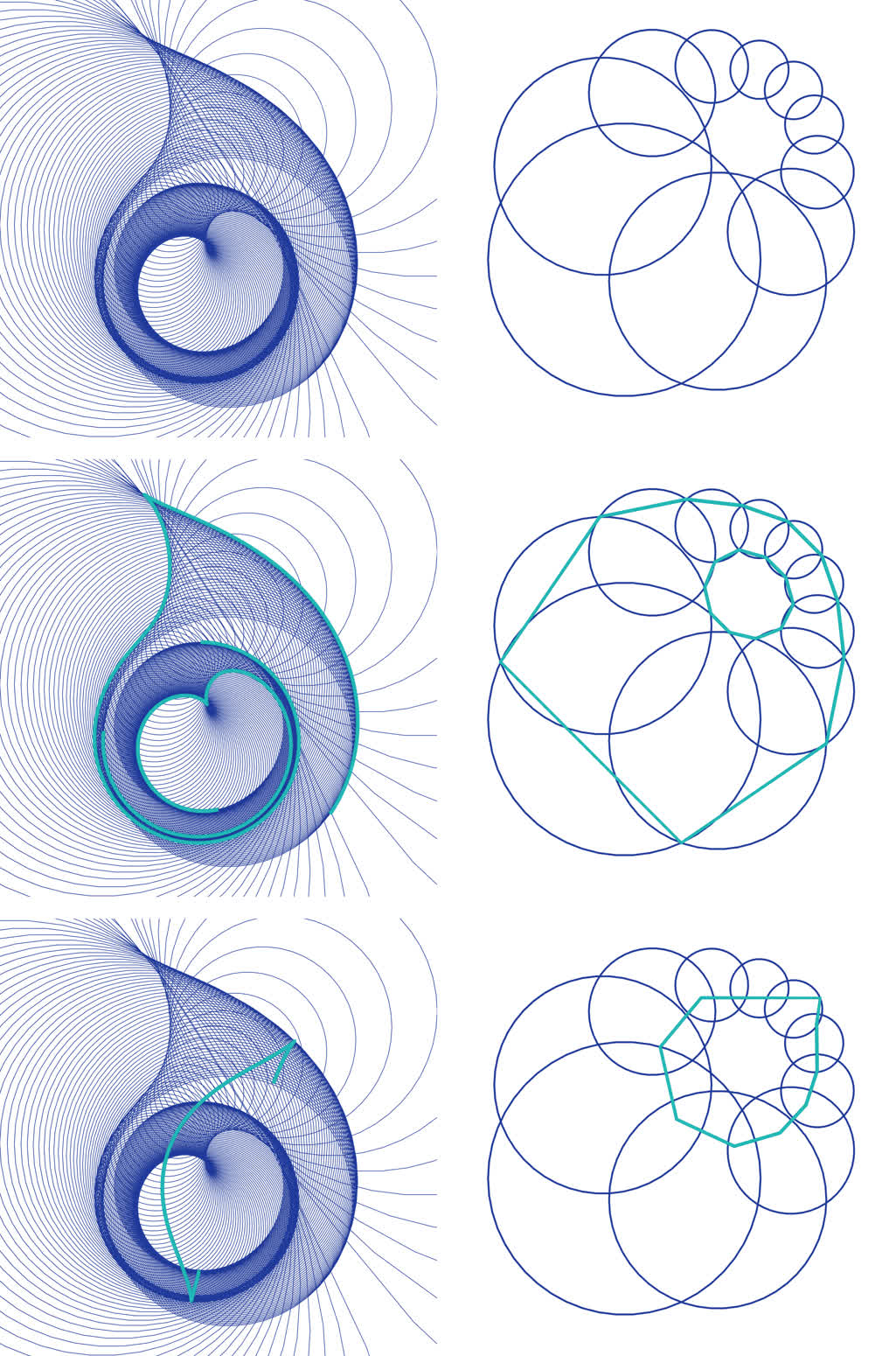
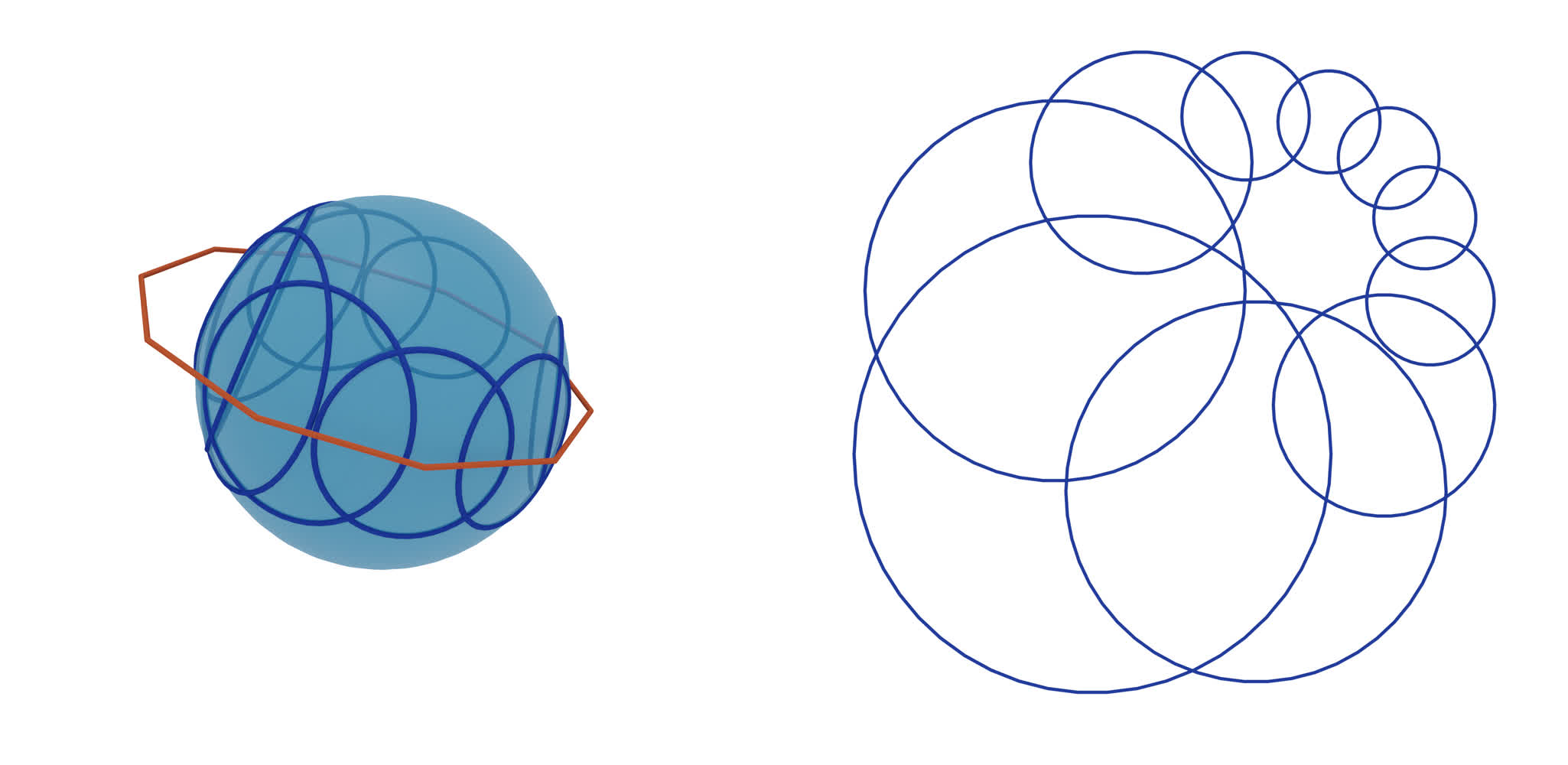
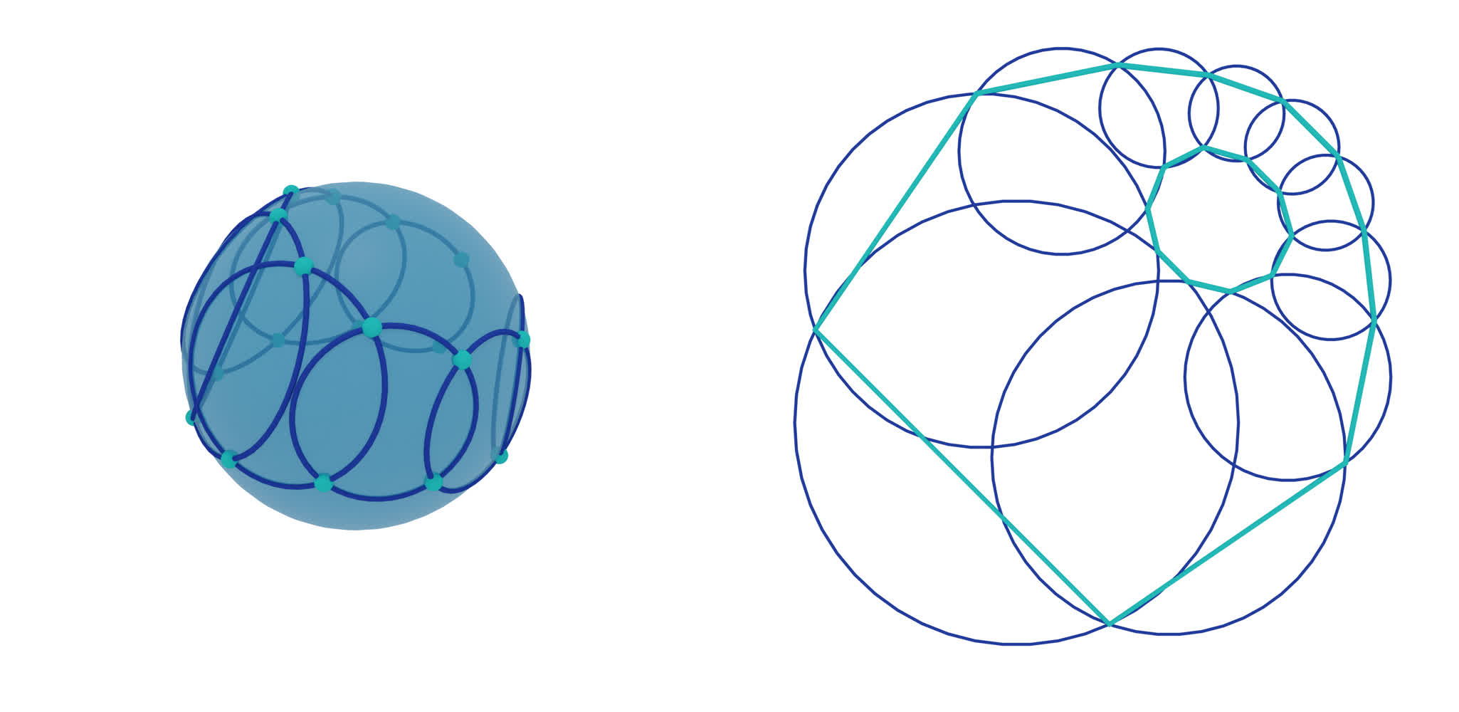
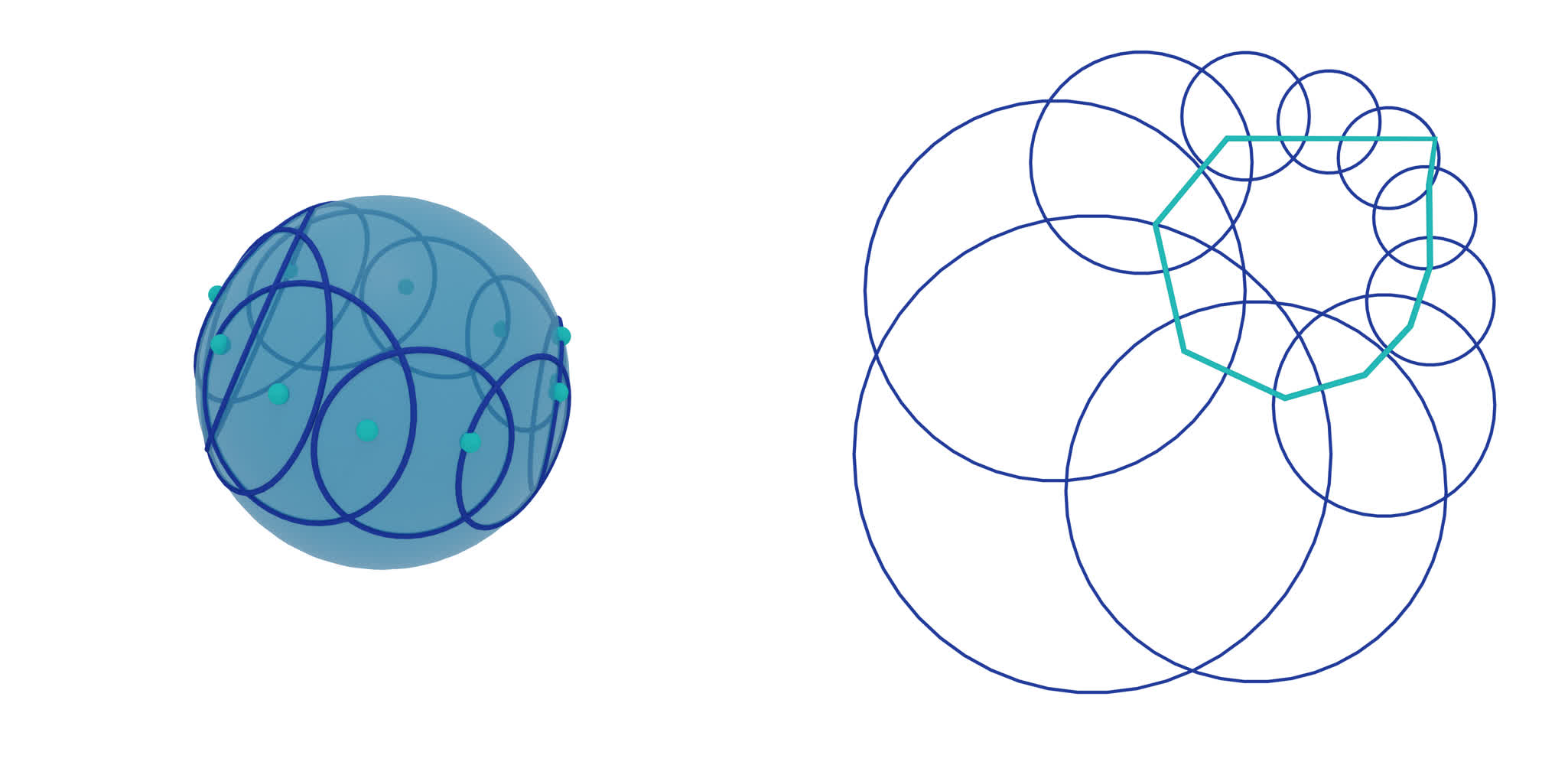
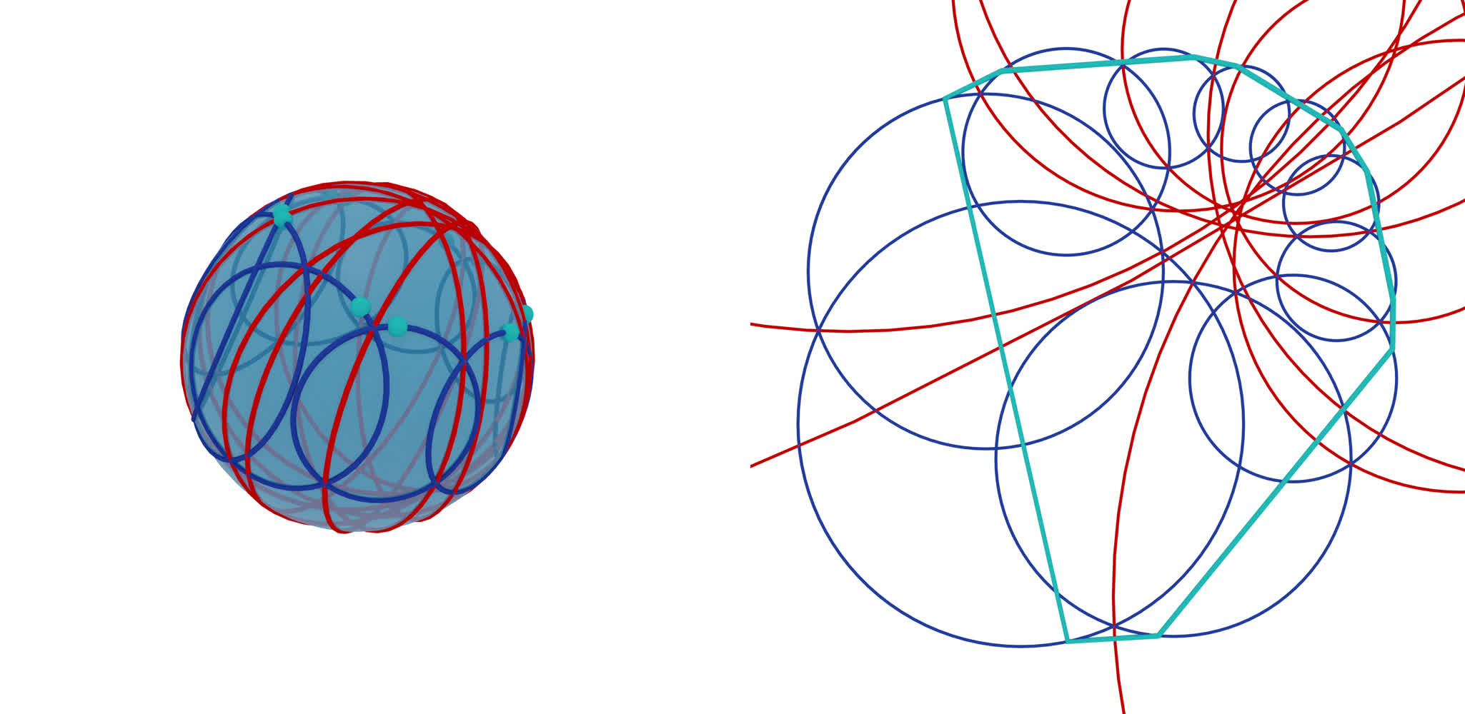
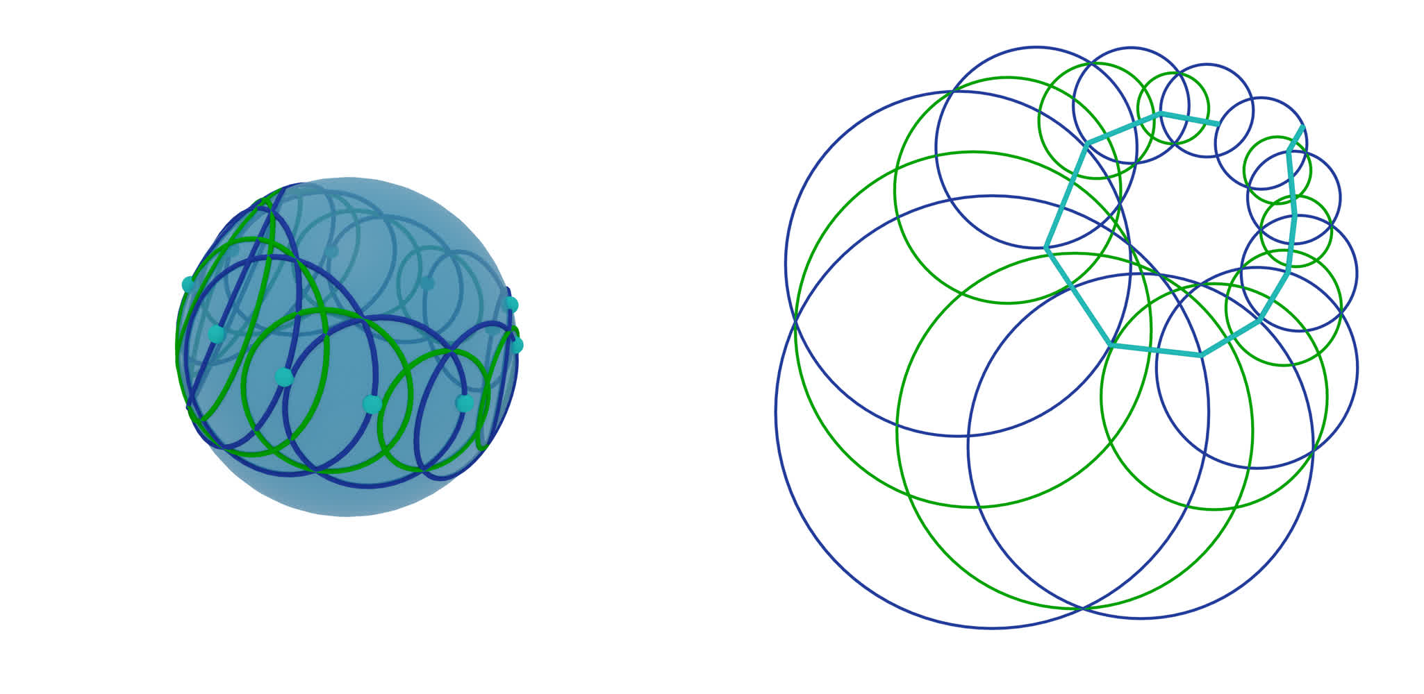
This example shows different ways of finding envelopes and orthogonal trajectories of a one-parameter family of circles, once in the smooth case and once in the discrete case. We start with a one-parameter family of circles where neighbouring circles intersect. The top left image shows a smooth family of circles, the top right image a discrete family of circles. The first envelope is constructed by connecting intersection points of consecutive circles. The first orthogonal trajectory is constructed by choosing an arbitrary starting point and iteratively applying sphere inversions in the circles. These two are shown in the second and third row of the image above. Secondly, envelopes and orthogonal trajectories are constructed by choosing a starting point on a circle and applying sphere inversions in the mid-circles of neighbouring circles. Executing the code in the script will visualize the smooth and the discrete examples, separated in distinct Blender collections. We will go through the discrete example in this guide.
Download the full script here:
envelope_orth_trajectory_circles.py.
Setup
We start off by importing the necessary libraries.
# Import necessary libraries
import numpy as np

import ddg
from ddg.blender.material import material
from ddg.geometry.euclidean_models import moebius_to_projective, projective_to_moebius
We are also going to clear the whole scene.
# Clear the existing objects in the Blender scene
ddg.blender.scene.clear()
ddg.blender.material.clear()
We initialize the projective and the Moebius geometric model of two dimensional Euclidean space.
euc = ddg.geometry.euclidean(2)
mob = ddg.geometry.euclidean_models.MoebiusModel(2)
First Envelope and Orthogonal Trajectory
The main script starts by defining a lot of helper functions. In the end the examples will be generated only by suitable composition of these functions. A lot of the functions are straight forward, and we will not explicitly include all of them here.
Now lets get started by defining a discrete curve outside the Moebius quadric \(M\) and some initial values.
    elif example == "discrete":
        # Conic section in M^+
        sampling_curve = 10
        h = ddg.geometry.Quadric(np.diag([0.8, 0.8, -1, -1]))
        p = ddg.geometry.hyperplane_from_normal([-1, -1, -5], level=-1)
        snet = ddg.to_smooth_net(ddg.geometry.intersect(h, p))
        dnet = ddg.nets.sample_smooth_net(snet, sampling=[sampling_curve, "t"])

        # Starting points of sphere inversions
        e_start_orth_1_phi = np.pi / 8
        e_start_orth_2_phi = np.pi / 8
        e_start_env_2_phi = np.pi / 8

        # Visualization
        bevel_curve = 0.03
        bevel_circle = 0.015
        circle_sampling = [0.1, 100, "c"]
        m_camera_location = (4, -3.3, 2.5)
        e_camera_location = (-1.2, -1.4, 10)

    else:
        raise Exception(f"{example = } has to be one of 'smooth' or 'discrete'")
The vertices of the discrete net are points outside the Moebius quadric (points with positive scalar square with respect to the Möbius scalar product) and therefore represent Euclidean circles. We can find the corresponding circles in the following way.
    ###############################################
    # Circles
    ###############################################

    # Moebius #####################################
    m_points_fct = function_affine_to_projective(dnet.fct)  # Points in M^+
    m_circles_fct = m_points_to_circles(m_points_fct)  # Conics in M

    # Euclidean ###################################
    e_circles_fct = project_function_of_objects_down(m_circles_fct)
The visualization is also done by using helper functions and can be found as the last section of this guide.
Next we want to create an envelope consisting of consecutive intersection points of circles. Inside the
helper function m_envelope we find a way of consistently determining the right
choice of the next intersection point (see script).
    ###############################################
    # Envelopes (as intersection points of circles)
    ###############################################

    # Moebius #####################################
    m_env_fct_0_0 = m_envelope(m_points_fct, index=0)  # Points in M
    m_env_fct_1_0 = m_envelope(m_points_fct, index=1)  # Points in M

    # Euclidean ###################################
    e_env_fct_0_0 = function_projective_to_affine(
        project_function_of_objects_down(m_env_fct_0_0)
    )  # affine coordinates
    e_env_fct_1_0 = function_projective_to_affine(
        project_function_of_objects_down(m_env_fct_1_0)
    )  # affine coordinates
For the first orthogonal trajectory we define a function representing a sphere inversion in a given circle.
Let \([c]\) be the representation of a circle as point outside of \(M\) and \([x]\) be a point on \(M\).
The formula \(x - 2 * \langle x, c \rangle / \langle c, c \rangle * c\) determines a point \(x'\), resp. \([x']\) in M,
which corresponds to the inversion of the point \(x\) in the circle \(c\).
Additionally the script supplies a function m_iterative_sphere_inversions,
applying this inversion iteratively to a family of circles.
    ###############################################
    # Orthogonal trajectory (inversion in circle family)
    ###############################################

    # Starting point ##############################
    circle0 = e_circles_fct(0)
    e_start_orth_1 = ddg.math.parametrizations.circle(
        e_start_orth_1_phi, circle0.center.affine_point, circle0.radius
    )  # Affine 3d coordinates
    m_start_orth_1 = projective_to_moebius(
        ddg.geometry.subspace_from_affine_points(e_start_orth_1)
    )  # Point in M

    # Moebius #####################################
    # Apply iterative inversions in the circles
    m_orth_fct_1 = m_iterative_sphere_inversions(
        m_points_fct, m_start_orth_1
    )  # Points in M

    # Euclidean ####################################
    e_orth_fct_1 = function_projective_to_affine(
        project_function_of_objects_down(m_orth_fct_1)
    )  # affine coordinates
Second Envelope and Orthogonal Trajectory
For the second envelope and orthogonal trajectory we need to find the mid-circles, the circle of
similitude and the circle of anti-similitude, between two neighbouring circles.
Circles with center \(c\) and radius \(r\) can explicitly be lifted
to the homogeneous coordinates \(\frac{1}{r}(c, \frac{1}{2}(||c||^2 - r^2 + 1) , \frac{1}{2}(||c||^2 - r^2 - 1))\), or
equivalently to \(\frac{1}{r}(c + e_0 + (||c||^2-r^2) e_\infty)\)
in the basis \(e_1, ...., e_3 e_0, e_\infty\).
If two circles are given in these homogeneous coordinates, say \(c\) and \(d\),
the mid-circles are represented by
\([c + d]\) and \([c-d]\). The two helper functions
m_points_of_similitude_from_homogeneous_lift and
m_points_of_anti_similitude_from_homogeneous_lift return these points while
the initial circles can be lifted using the function m_homogeneous_lift_fct.
    ###############################################
    # Circles of similitude and anti-similitude
    ###############################################

    # Moebius #####################################
    m_homogeneous_points_fct = m_homogeneous_lift_fct(
        e_circles_fct
    )  # Homogeneous coordinates in R^{3, 1}
    m_points_of_similitude_fct = m_points_of_similitude_from_homogeneous_lift(
        m_homogeneous_points_fct
    )  # Points in M+
    m_circles_of_similitude_fct = m_points_to_circles(
        m_points_of_similitude_fct
    )  # Conics in M
    m_points_of_anti_similitude_fct = m_points_of_anti_similitude_from_homogeneous_lift(
        m_homogeneous_points_fct
    )  # Homogeneous coordinates in R^{3, 1}
    m_circles_of_anti_similitude_fct = m_points_to_circles(
        m_points_of_anti_similitude_fct
    )  # Conics in M

    # Euclidean ####################################
    e_circles_of_similitude_fct = project_function_of_objects_down(
        m_circles_of_similitude_fct
    )  # Circles in R2 in R3
    e_circles_of_anti_similitude_fct = project_function_of_objects_down(
        m_circles_of_anti_similitude_fct
    )  # Circles in R2 in R3
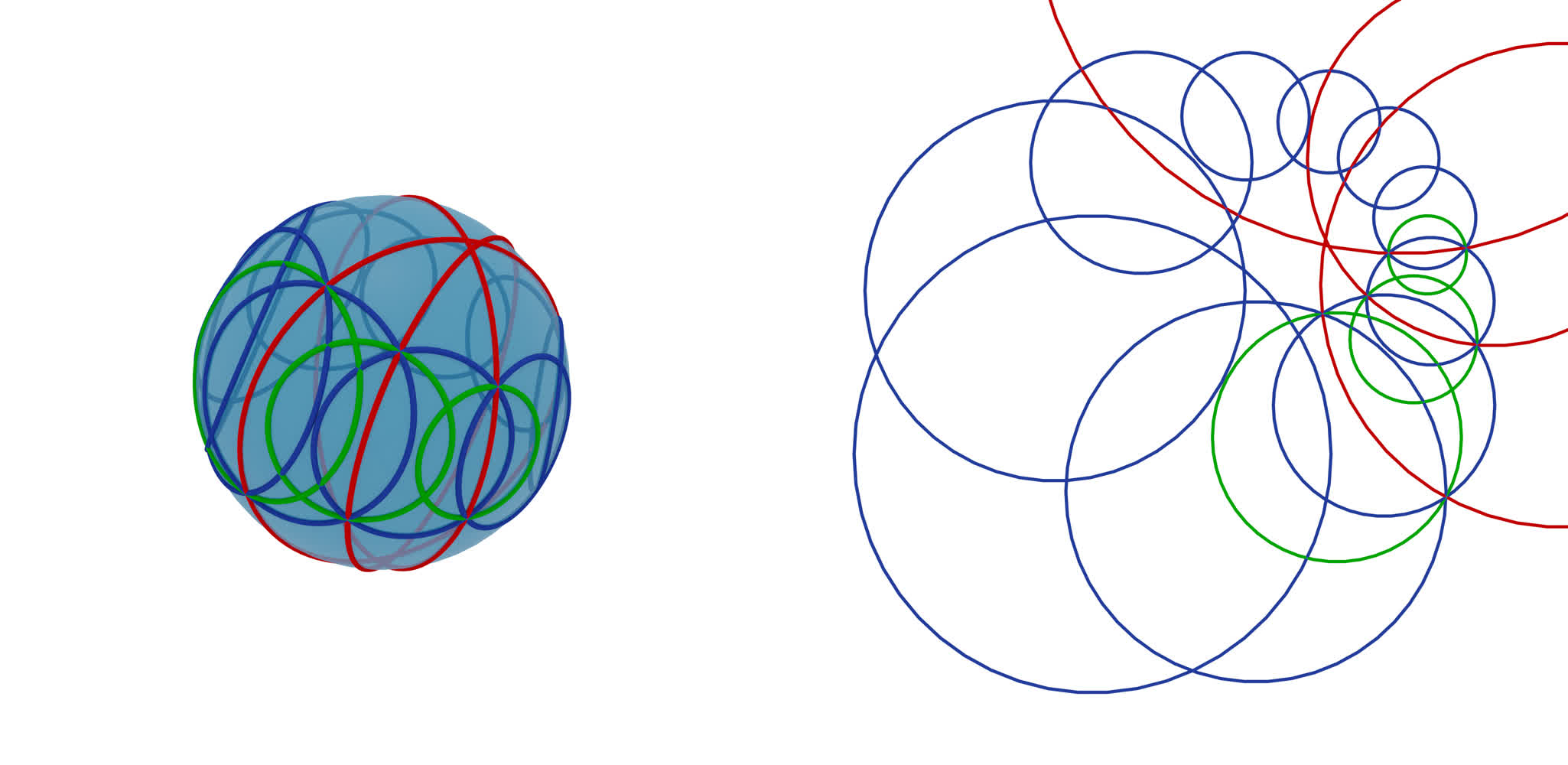
With this it is easy to define the corresponding envelopes and orthogonal trajectories.
    ###############################################
    # Envelope (as sphere inversions in circles of anti-similitude)
    ###############################################

    # Starting point ##############################
    e_start_env_2 = ddg.math.parametrizations.circle(
        e_start_env_2_phi, circle0.center.affine_point, circle0.radius
    )  # affine_coordinates
    m_start_env_2 = projective_to_moebius(
        ddg.geometry.subspace_from_affine_points(e_start_env_2)
    )  # Point in M

    # Moebius #####################################
    m_env_fct_2 = m_iterative_sphere_inversions(
        m_points_of_anti_similitude_fct, m_start_env_2
    )  # Points in M

    # Euclidean ####################################
    e_env_fct_2 = function_projective_to_affine(
        project_function_of_objects_down(m_env_fct_2)
    )  # affine coordinates
    ###############################################
    # Orthogonal trajectory (as sphere inversions in circles of similitude)
    ###############################################

    # Starting point ##############################
    e_start_orth_2 = ddg.math.parametrizations.circle(
        e_start_orth_2_phi, circle0.center.affine_point, circle0.radius
    )  # affine_coordinates
    m_start_orth_2 = projective_to_moebius(
        ddg.geometry.subspace_from_affine_points(e_start_orth_2)
    )  # Point in M

    # Moebius #####################################
    m_orth_fct_2 = m_iterative_sphere_inversions(
        m_points_of_similitude_fct, m_start_orth_2
    )

    # Euclidean ####################################
    e_orth_fct_2 = function_projective_to_affine(
        project_function_of_objects_down(m_orth_fct_2)
    )  # affine coordinates
Visualization
With all this setup done, we can now visualize this in Blender. We start by defining some colors and helper functions. For some functions the discrete domain may be clipped at the start or at the end. For this we also use a helper function.
################################################
# Visualization setup
################################################
orange = material("orange", (0.8, 0.1, 0.036), 0, 0)
red = material("red", (1.0, 0.0, 0.0), 0, 0)
green = material("green", (0.0, 0.5, 0.0), 0, 0)
blue = material("blue", (0.019, 0.052, 0.445), 0, 0)
turquoise = material("turquoise ", (0.02, 0.8, 0.77), 0, 0)
transparency_sphere = 0.6
transparent_sphere = ddg.blender.material.material(
    "transparent_sphere", (0.018, 0.313, 0.656), 0.5, 0.5, alpha=transparency_sphere
)


def visualize_circles(g, domain, name, material=None, collection=None):
    l = []
    for i in range(*domain[0]):
        bobj = ddg.blender.convert(g(i), f"{name}_{i}", material, collection)
        bobj.data.bevel_depth = bevel_circle
        l.append(bobj)

    return l


def visualize_pts(g, domain, name, material=turquoise, collection=None):
    return [
        ddg.blender.convert(
            g(i),
            f"{name}_{i}",
            material,
            collection,
        )
        for i in range(*domain[0])
    ]


def visualize_curve(dnet_fct, domain, name, material=None, collection=None):
    dnet = ddg.nets.DiscreteNet(dnet_fct, domain=domain)
    bobj = ddg.blender.convert(dnet, name, material, collection)
    bobj.data.bevel_depth = bevel_curve
    return bobj


def shift_domain(a, b, domain):
    return [[domain[0][0] + a, domain[0][1] + b]]
For each example (“smooth”/”discrete”) we add a set of collections …
    mob_col = ddg.blender.collection.collection(
        f"Moebius_{example}",
        children=[
            f"m_circles_{example}",
            f"m_envelope_1_{example}",
            f"m_orthogonal_trajectory_1_{example}",
            f"m_envelope_2_{example}",
            f"m_orthogonal_trajectory_2_{example}",
        ],
    )

    euc_col = ddg.blender.collection.collection(
        f"Euclidean_{example}",
        children=[
            f"e_circles_{example}",
            f"e_envelope_1_{example}",
            f"e_orthogonal_trajectory_1_{example}",
            f"e_envelope_2_{example}",
            f"e_orthogonal_trajectory_2_{example}",
        ],
    )
… and visualize the Moebius geometric part …
    ###############################################
    # Moebius
    ###############################################
    mob_curve = ddg.blender.convert(dnet, "mob_curve", orange, mob_col)
    mob_curve.data.bevel_depth = 0.015
    mob_quadric_bobj = ddg.blender.convert(
        mob.absolute,
        "mob_quadric",
        transparent_sphere,
        mob_col,
    )
    ddg.blender.mesh.shade_smooth(mob_quadric_bobj)

    #  dnet.domain = ddg.nets.DiscreteDomain([[*dnet.domain[0]]])
    # # circles
    visualize_circles(
        m_circles_fct,
        domain=shift_domain(0, 1, dnet.domain),
        name="m_circle",
        material=blue,
        collection=mob_col.children[0],
    )

    # envelopes 1 (intersection points)
    visualize_pts(
        m_env_fct_0_0,
        domain=dnet.domain,
        name="m_env_1_point_0",
        collection=mob_col.children[1],
    )
    visualize_pts(
        m_env_fct_1_0,
        domain=dnet.domain,
        name="m_env_1_point_1",
        collection=mob_col.children[1],
    )

    # orthogonal_trajectories 1
    visualize_pts(
        m_orth_fct_1,
        domain=shift_domain(1, 3, dnet.domain),
        name="m_orth_traj_1_point",
        collection=mob_col.children[2],
    )

    # envelopes 2 (circles of anti similitude)
    visualize_circles(
        m_circles_of_anti_similitude_fct,
        domain=dnet.domain,
        name="m_circle_of_anti_similitude",
        material=red,
        collection=mob_col.children[3],
    )
    visualize_pts(
        m_env_fct_2,
        domain=shift_domain(0, 3, dnet.domain),
        name="m_env_2_point",
        collection=mob_col.children[3],
    )

    # orthogonal trajectories 2
    visualize_circles(
        m_circles_of_similitude_fct,
        domain=dnet.domain,
        name="m_circle_of_similitude",
        material=green,
        collection=mob_col.children[4],
    )
    visualize_pts(
        m_orth_fct_2,
        name="m_orth_traj_2_point",
        domain=shift_domain(0, 2, dnet.domain),
        collection=mob_col.children[4],
    )
… and the Euclidean part.
    ###############################################
    # Euclidean
    ###############################################
    # circles
    visualize_circles(
        e_circles_fct,
        domain=shift_domain(0, 1, dnet.domain),
        name="e_circle",
        material=blue,
        collection=euc_col.children[0],
    )

    # envelopes 1 (intersection points)
    visualize_curve(
        e_env_fct_0_0,
        domain=shift_domain(0, 1, dnet.domain),
        name="e_env_1_0",
        material=turquoise,
        collection=euc_col.children[1],
    )
    visualize_curve(
        e_env_fct_1_0,
        domain=shift_domain(0, 1, dnet.domain),
        name="e_env_1_1",
        material=turquoise,
        collection=euc_col.children[1],
    )

    # orthogonal_trajectories 1
    visualize_curve(
        e_orth_fct_1,
        domain=shift_domain(0, 2, dnet.domain),
        name="e_orth_traj_1",
        material=turquoise,
        collection=euc_col.children[2],
    )

    # envelopes 2 (cirlces of anti similitude)
    visualize_circles(
        e_circles_of_anti_similitude_fct,
        domain=dnet.domain,
        name="e_circle_of_anti_similitude",
        material=red,
        collection=euc_col.children[3],
    )
    visualize_circles(
        e_circles_of_similitude_fct,
        domain=dnet.domain,
        name="e_circle_of_similitude",
        material=green,
        collection=euc_col.children[4],
    )
    visualize_curve(
        e_env_fct_2,
        domain=dnet.domain,
        name="e_env_2",
        collection=euc_col.children[3],
        material=turquoise,
    )

    # orthogonal trajectories 2
    visualize_curve(
        e_orth_fct_2,
        domain=shift_domain(0, 1, dnet.domain),
        name="e_orth_traj_2",
        material=turquoise,
        collection=euc_col.children[4],
    )
The script further includes adding lights and cameras and setting up the scene for rendering.