Minimal (Maximal) Surfaces from Weierstrass Data – The Catenoid

In this example, we will construct discrete S-isothermic minimal surfaces from discrete Weierstrass data. We can use the same code to construct spacelike S-isothermic maximal surfaces in Lorentz-Minkowski space \(\mathbb{R}^{2,1}\), the analogue of minimal surfaces in Lorentz-Minkowski space.

For background information we refer to the paper [BHS06: Minimal surfaces from circle patterns] and the papers [ADMPS24: Discrete Lorentz surfaces and s-embeddings I & II].

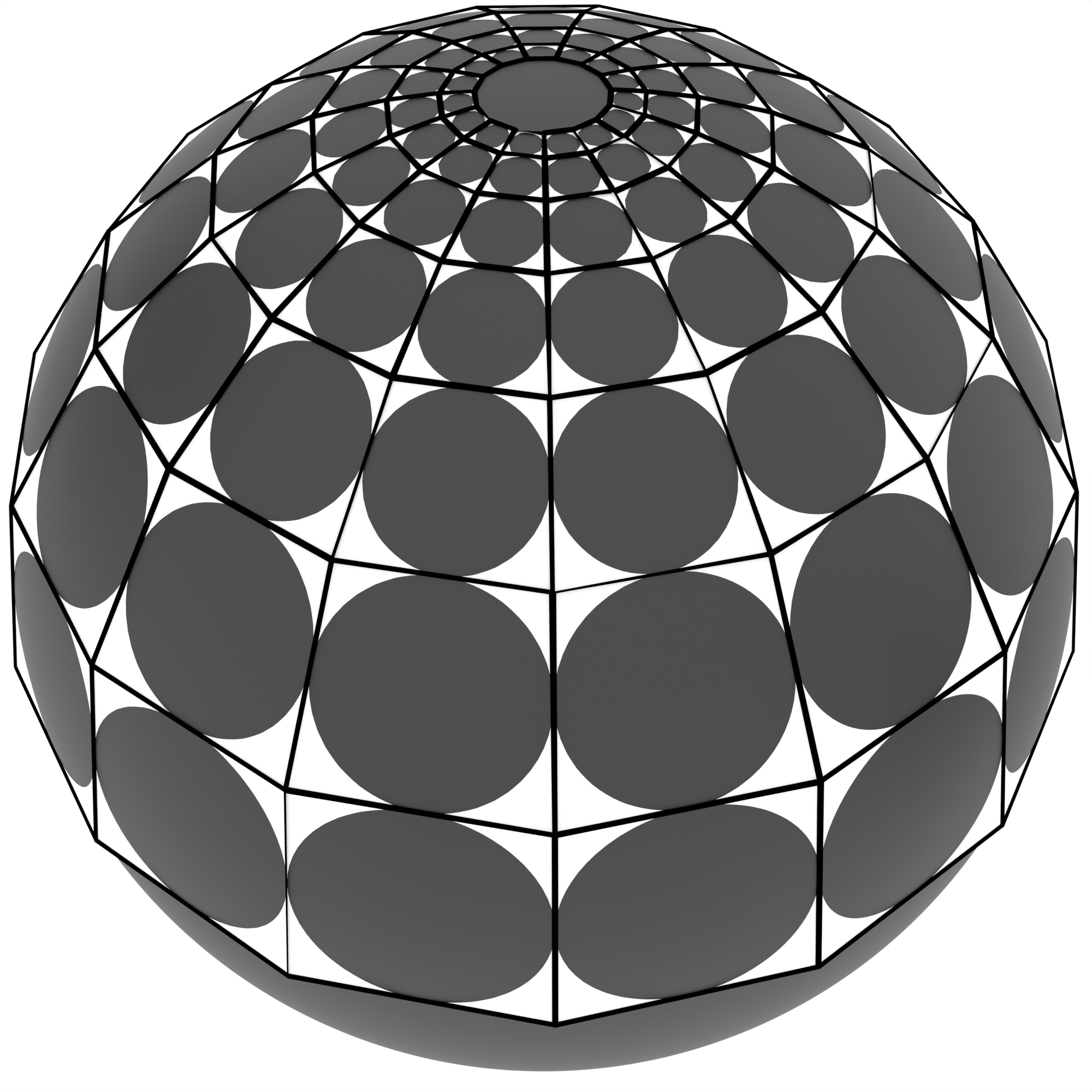
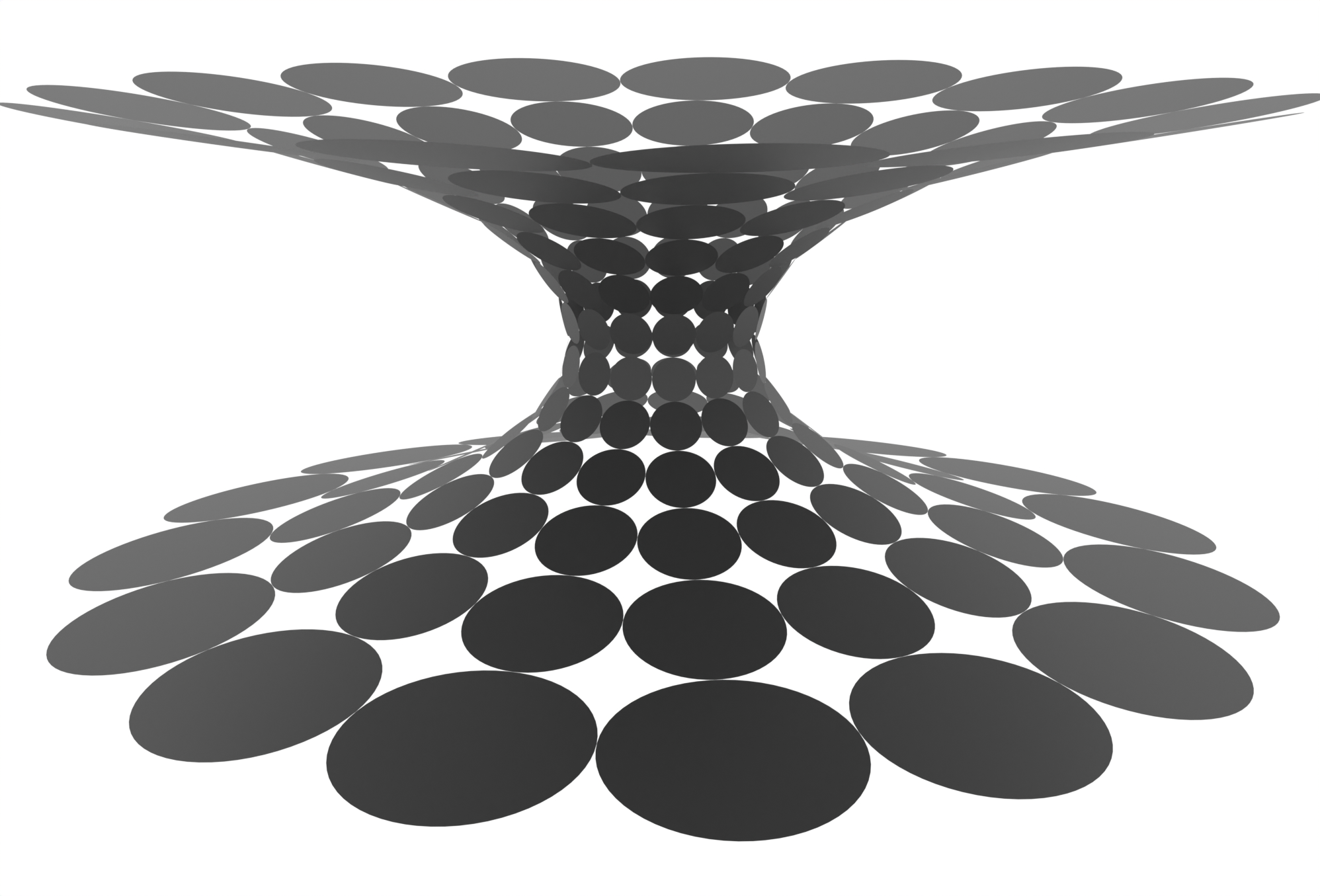
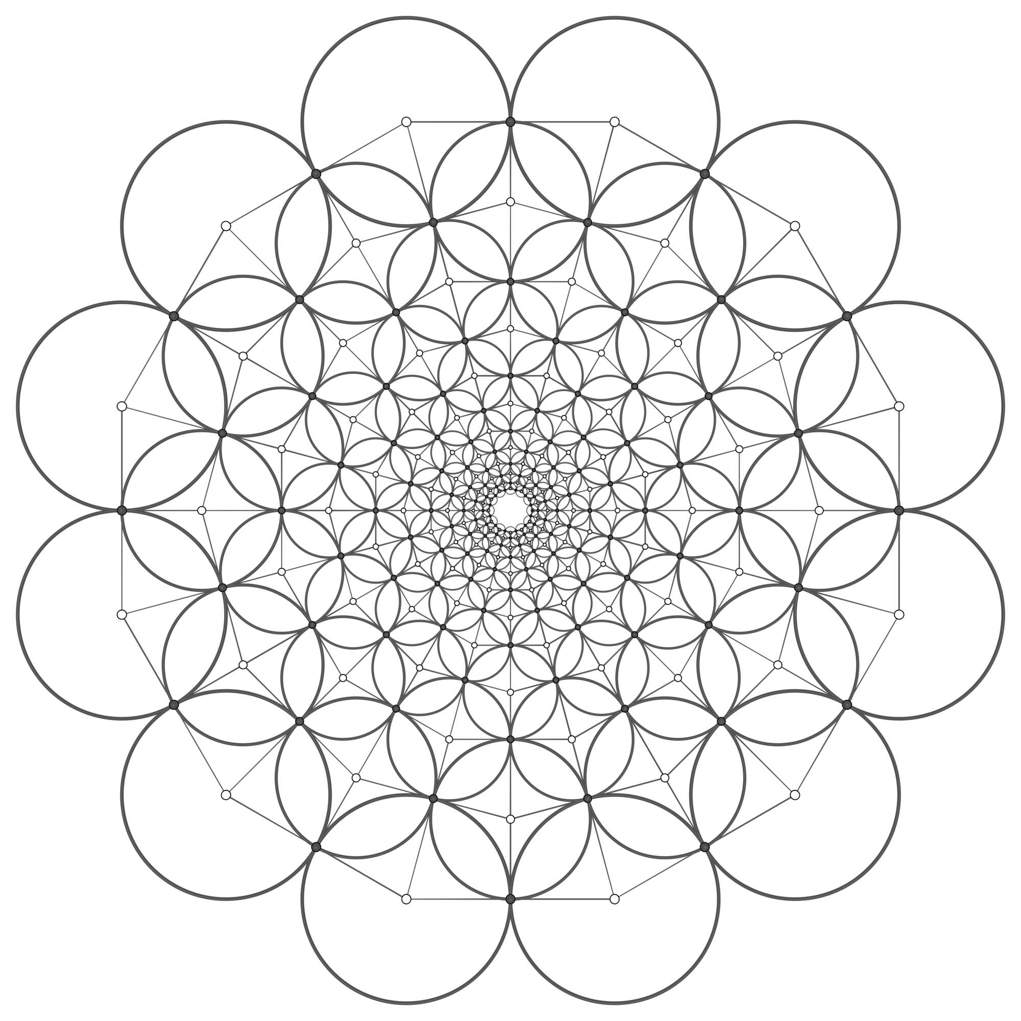
We will use the S-Exp circle pattern, shown below, from this example as discrete Weierstrass data. We could use the explicit Weierstrass representation formula, but instead we will project the S-Exp circle pattern to a Koebe net tangential to the unit sphere, and Christoffel dualize it to obtain a discrete S-isothermic surface. For the S-Exp circle pattern the resulting S-isothermic surface will be a discrete catenoid.

You can download the full script minimal_catenoid.py and obj files storing the central extension (see below) of the catenoid in Euclidean catenoid_euc.obj or Lorentz-Minkowski space catenoid_lor.obj.

Setup

We begin by importing the required modules, clearing the Blender scene, and defining the unit sphere and the dot product.

# From discrete Weierstrass data (orthogonal circle pattern)
# to an S-isothermic minimal surface
import os

import bpy
import numpy as np

import ddg

# Clear the Blender scene
ddg.blender.scene.clear(deep=True)

geo = "euc"
# geo = "lor"

if geo == "euc":
    us = ddg.geometry.Quadric(np.diag([1.0, 1.0, 1.0, -1.0]))

    def dot(u, v):
        return u[0] * v[0] + u[1] * v[1] + u[2] * v[2]


if geo == "lor":
    us = ddg.geometry.Quadric(np.diag([1.0, 1.0, -1.0, 1.0]))

    def dot(u, v):
        return u[0] * v[0] + u[1] * v[1] - u[2] * v[2]


# Point of stereographic projection
N = ddg.geometry.Point([0, 0, -1.0, 1.0])

This example can easily be modified to create a maximal surface in Lorentz-Minkowski space. We simply need to choose the geometry to be "lor".

We load the Weierstrass data (for \(\mathbb{R}^{2,1}\) it must lie inside the Poincaré disc) from an .obj file. Its vertices divide into white and black vertices, corresponding to cirlce centers and touching points respectively.

# ================================================================
# Load data
# ================================================================
# Note that for the Lorentz setup, to handle vertices at infinity,
# we need an s-exp pattern initialized with an odd U.
dir = os.path.dirname(os.path.realpath(__file__))
combinatorics = ddg.conversion.halfedge.obj.obj_to_hds(f"{dir}/s_exp.obj")

Preparation

We prepare our data. We color the vertices and black and white (b and w), and the white ones again in ws and wc vertices. The bi-coloring of the white vertices distinguishes which white vertices will become spheres (ws) and which will become circles (wc) of the S-isothermic surface. The black vertices will be the touching points.

# ================================================================
# Color vertices
# ================================================================
# Divide vertices in black and white vertices and the white ones again, to
# distinguish which will become spheres and which will become circles.
ddg.halfedge.bicolor_vertices(combinatorics, colors=["w", "b"])
white_verts = [v for v in combinatorics.verts if v.color == "w"]
black_verts = [v for v in combinatorics.verts if v.color == "b"]

verts = sorted(list(combinatorics.verts), key=lambda v: v.index)
white_net = ddg.halfedge.diagonals(combinatorics)[0]
assert verts[ddg.halfedge.some_vertex(white_net).old_index].color == "w"

ddg.halfedge.bicolor_vertices(white_net, colors=["ws", "wc"])
combinatorics.verts.add_attribute("white_type", None)
for v in white_net.verts:
    verts[v.old_index].white_type = "wc" if v.color == "wc" else "ws"

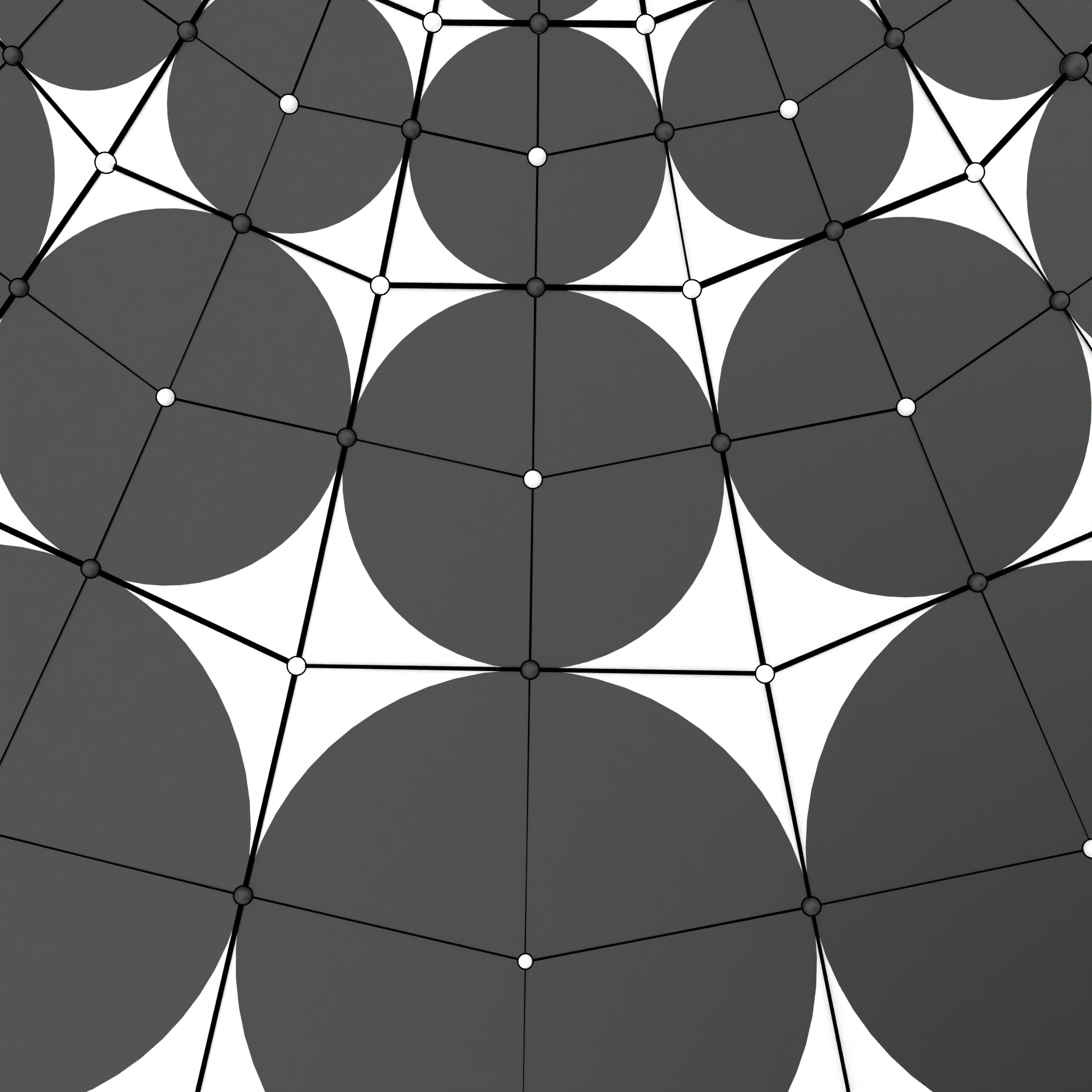
Project to a Koebe net

We want to construct an S-isothermic Koebe net, tangential to the unit sphere, with white sphere centers ws and white circle centers wc. For the Koebe net, black points will be the points of tangency, so we project all of the black points to the unit sphere. We can compute all of the white points to be the the points polar to the planes that contain all adjacent black points. For the sphere centers ws these are the correct points. For the circle centers wc there is an easy formula to obtain the correct points from the polar points we have constructed before.

# ================================================================
# Project to Koebe net
# ================================================================
# Construct the central extension of a Koebe net: black vertices are
# the points of tangency, they lie in 'us'. White 'ws' vertices are
# sphere centers outside of 'us' and white 'wc' are circle centers inside 'us'.
combinatorics.verts.add_attribute("koebe_co")

for b in black_verts:
    proj = ddg.geometry.inverse_stereographic_project(
        ddg.geometry.Point([*b.co, 1], atol=1e-15, rtol=0.0), us, N
    )
    b.koebe_co = proj.affine_point

for w in white_verts:
    neighbors = [e.head for e in ddg.halfedge.out_edges(w)]
    plane = ddg.geometry.subspace_from_affine_points(
        *[b.koebe_co for b in neighbors], atol=1e-15, rtol=0.0
    )
    w.koebe_co = us.polarize(plane).affine_point
    if w.white_type == "wc":
        w.koebe_co = w.koebe_co / np.abs(dot(w.koebe_co, w.koebe_co))

Dualize

Now we want to compute the Christoffel dual of the Koebe net. It is known that the central extension of an S-isothermic surface is a discrete isothermic (factorizing face cross-ratio) surface. The discrete one-form for the Christoffel dual of an isothermic surface is \(\partial c^* (v, v') = \pm \frac{\partial c (v, v') }{|\partial c (v, v') |^2}\) for all edges \((v, v')\). We initialize the Christoffel dual by associating new edges to the old ones, which we determine by the formula above. We also need to bi-color the edges, as half the edges change direction in the Christoffel dual. We can verify that the one-form closes, and then integrate it by specifying a starting vertex, its position, and the name of the new vertex attribute to store the coordinates of the dual surface. Note that we also multiply by a global scaling.

# ================================================================
# Christoffel dual
# ================================================================
# Set attribute storing edges of the Christoffel dual (with global scaling)
ddg.halfedge.bicolor_edges(combinatorics, "color", [1, -1])
combinatorics.edges.add_attribute("new_edge")

for e in combinatorics.edges:
    diff = e.head.koebe_co - e.tail.koebe_co
    normsq = dot(diff, diff)
    e.new_edge = (1 / normsq) * diff * e.color / 70

# Define boundary vertices where the integration of the one-form stops proceeding
combinatorics.verts.add_attribute("bdy")
for v in combinatorics.verts:
    if ddg.halfedge.is_boundary_vertex(v) and np.isclose(np.linalg.norm(v.co), 1.0):
        v.bdy = True

# Construct Christoffel dual
ddg.halfedge.verify_closure_one_form(combinatorics, "new_edge")
combinatorics = ddg.halfedge.integrate_one_form(
    combinatorics,
    ddg.halfedge.some_vertex(combinatorics),
    np.array([1.0, 2.5, 1.5]),
    "dual_co",
    "new_edge",
    boundary_attr="bdy",
)

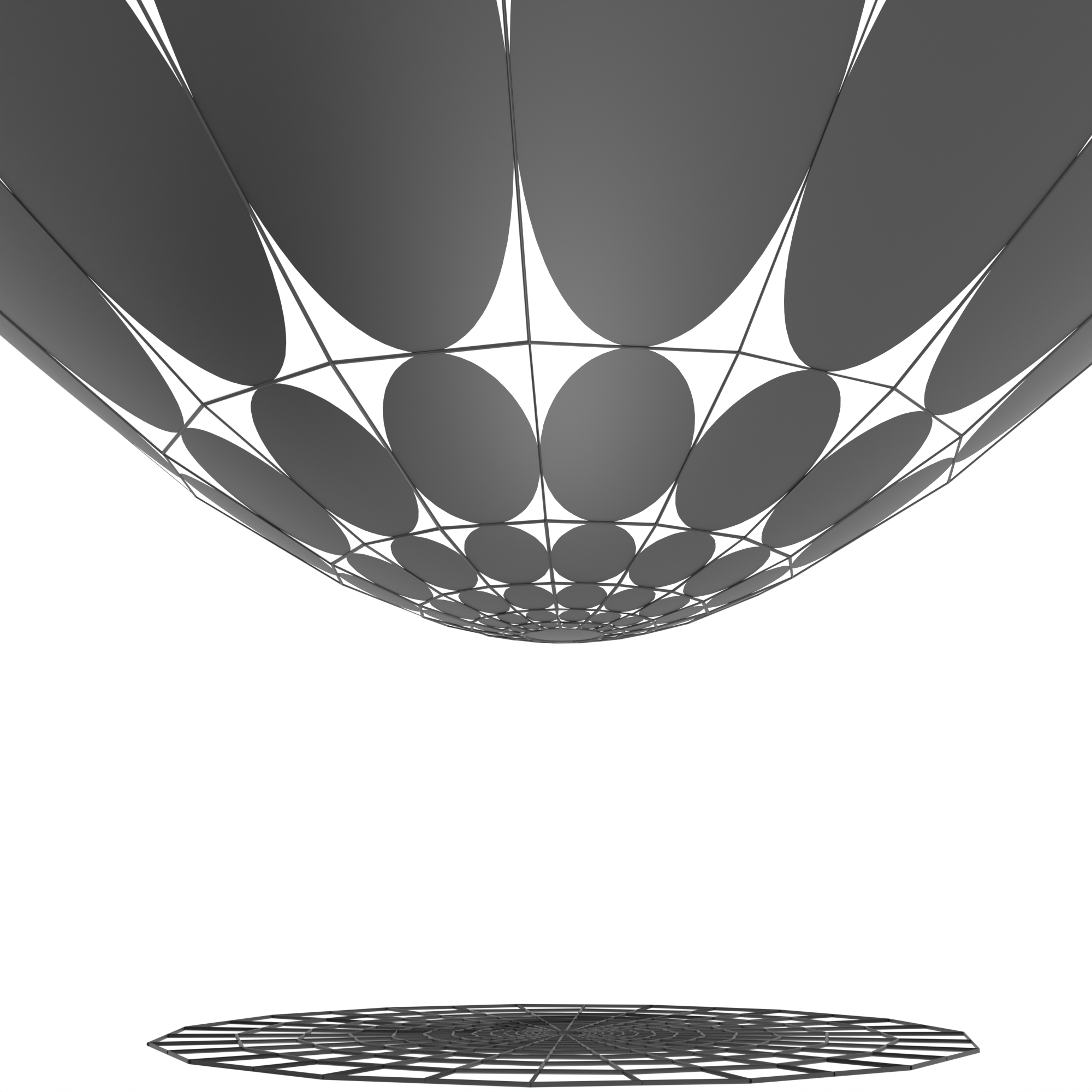
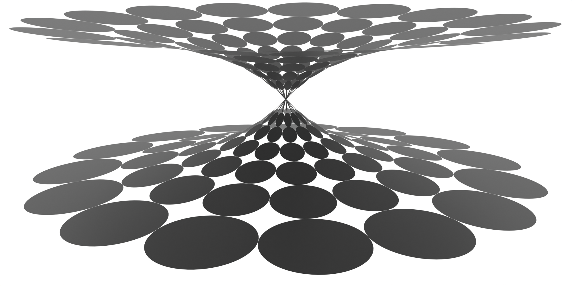
The resulting maximal surface is the central extension of an S-isothermic surface. One family of white vertices forms the S-isothermic surface. The other white vertices are again the circle centers.

Note that the resulting surfaces are only half of the catenoid. The other half can be obtained by reflection a plane parallel to the xy plane. For the visualization of the images we simply applied this reflection in Blender.

Visualization

In the visualization step, we can render various objects. For a more detailed visualization of the s_exp circle pattern, see the s-exp example.

# ================================================================
# Visualize
# ================================================================
primal = ddg.halfedge.diagonals(ddg.halfedge.diagonals(combinatorics)[0])[0]

black = ddg.blender.material.material(color=(0.0, 0.0, 0.0), name="black")
white = ddg.blender.material.material(color=(1.0, 1.0, 1.0), name="white")

ddg.blender.edges(combinatorics, "s_exp", radius=0.005, material=black)

bobj_us = ddg.blender.convert(
    ddg.arrays.from_quadric(us, (100, 0.125), (100, 0.125)),
    "unit_sphere",
    material=black,
)
with ddg.blender.bmesh.bmesh_from_mesh(bobj_us.data) as bm:
    ddg.blender.bmesh.cut_bounding_box(
        bm, np.array([np.inf, np.inf, 3]), np.array([0, 0, 2])
    )

ddg.blender.convert(
    ddg.arrays.from_half_edge_surface(primal, "koebe_co"),
    "koebe_primal",
    material=white,
)
ddg.blender.edges(
    ddg.arrays.from_half_edge_surface(primal, "koebe_co"),
    "koebe_edges",
    radius=0.005,
    material=black,
)

# ddg.blender.convert(
#    ddg.arrays.from_half_edge_surface(primal, "dual_co"), "max_primal", material=white
# )

ddg.blender.edges(
    ddg.arrays.from_half_edge_surface(primal, "dual_co"),
    "max_primal_edges",
    radius=0.005,
    material=black,
)

We can also visualize the touching face circles of the surface in a way that works for the Euclidean as well as for the Lorentzian case.

# ================================================================
# Visualize face circles
# ================================================================
# For an orthonormal basis (u,w) of a planar face we can use a circle
# parameterization function to compute the incircle
# of the face and convert it to a disc.
for v in combinatorics.verts:
    if v.white_type == "wc" and not ddg.halfedge.is_boundary_vertex(v):
        e = next(ddg.halfedge.out_edges(v))
        u = e.head.dual_co - v.dual_co
        w = e.nex.head.dual_co - e.head.dual_co

        u /= np.sqrt(dot(u, u))
        w /= np.sqrt(dot(w, w))

        r = np.mean(
            [
                np.sqrt(dot(v.dual_co - e.head.dual_co, v.dual_co - e.head.dual_co))
                for e in ddg.halfedge.out_edges(v)
            ]
        )

        def circle(theta):
            return v.dual_co + r * np.cos(theta) * u + r * np.sin(theta) * w

        cos = [circle(t) for t in np.arange(0, 2 * np.pi, 0.1)]

        disc = ddg.halfedge.Surface()
        disc.add_face(len(cos))
        disc.verts.add_attribute("co")
        for vert in disc.verts:
            setattr(vert, "co", cos[vert.index])

        ddg.blender.convert(disc, f"face_circle_{v.index}", material=black)

OBJ Export and Rendering Setup

The remaining part of the file contains code for exporting an OBJ file and setting up rendering options.