Caustics
This example visualizes mathematical and physical caustics. It shows how to construct and visualize a planar caustic with variable reflection curve and light source. We construct the mathematical caustics as the enveloppe of the reflection of light rays on a curve. The physical caustics are simulated using Blender’s built-in raytracer Cycles.
The curves in this example are discrete arcs of a circle.
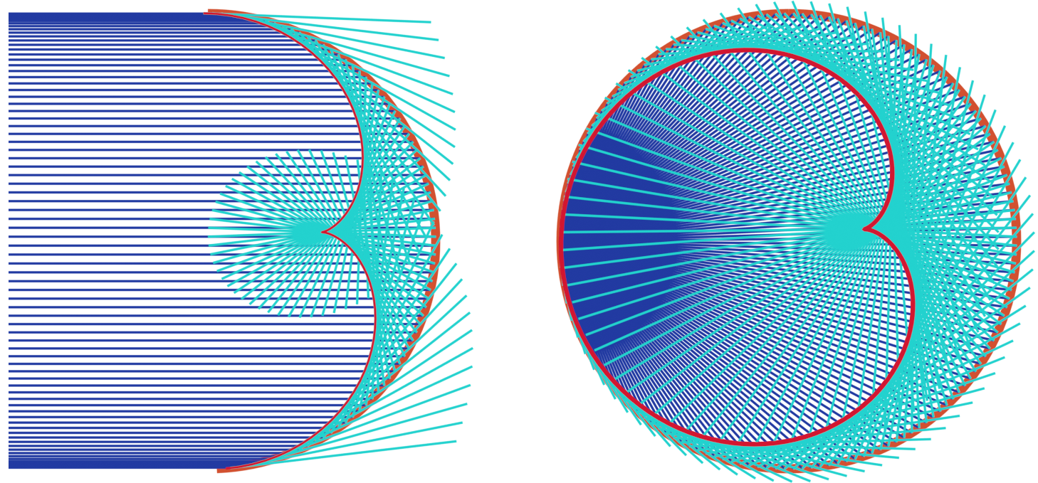
The example includes 2 mathematical constructions:
Parallel incoming light rays reflected on an half circle result in a nephroid caustic.
Radial incoming light rays orgiginated from a point on a circle result in a cardioid caustic.

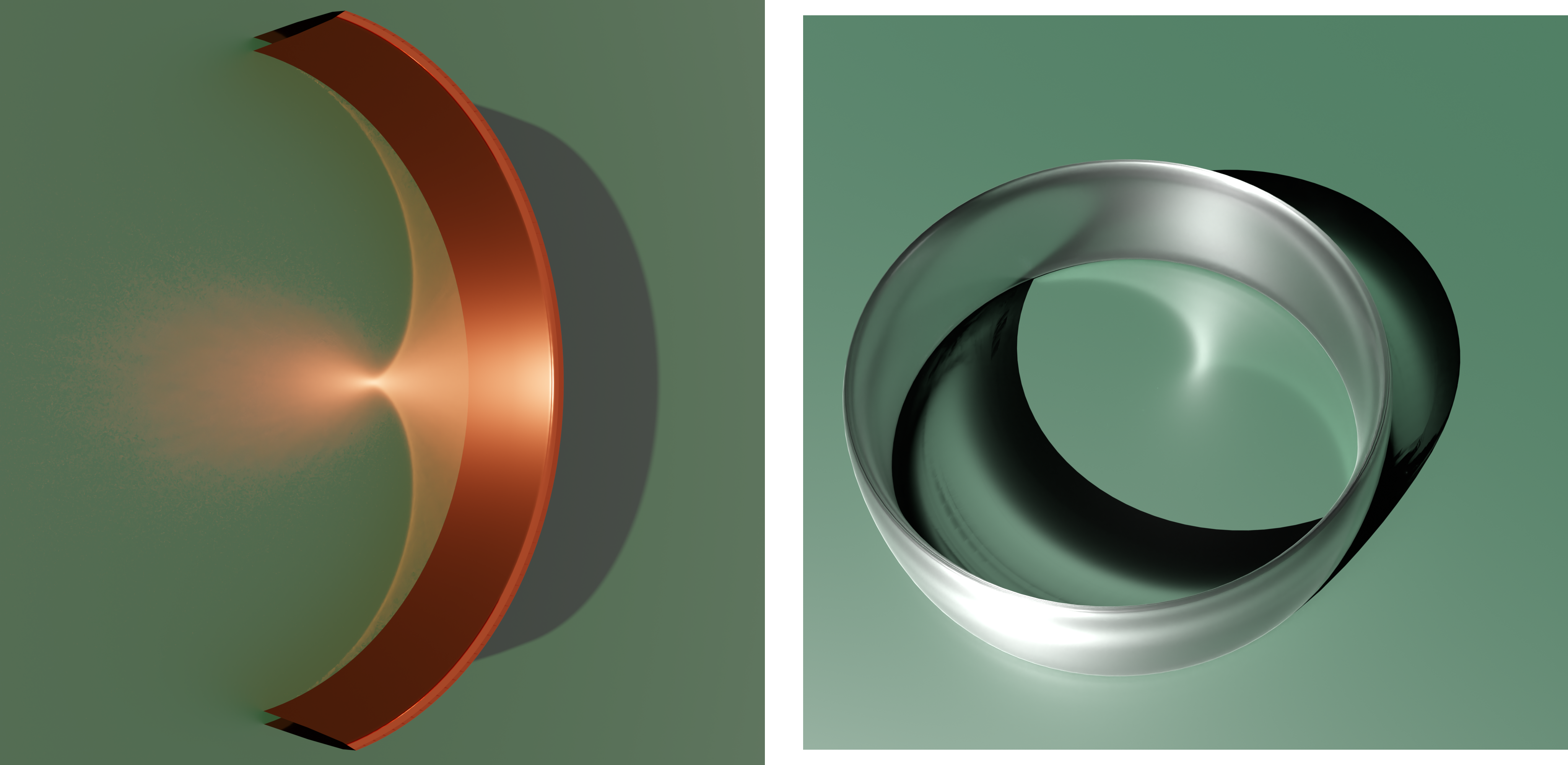
Furthermore this example includes a physical simulating of the first construction.
You can download the full script
caustics.py,
or find it, separated in sections, below.
Be aware that the example, at the end, contains settings for internal snapshot testing.
Comment or remove these to apply the actual (rendering) settings of the example.
Setup
#################
# Initial setup #
#################

ddg.visualization.blender.scene.clear()

collection_mathematical = ddg.visualization.blender.collection.collection(
    "theoretic_caustics", children=["cardioid", "nephroid"]
)
collection_physical = ddg.visualization.blender.collection.collection("real_caustics")
Helper Functions
Functions for creation of planar and spherical curvature circles and projections of objects (per index).
####################
# Helper functions #
####################


def edge_midpoints(fct):
    """Returns a function that returns the midpoint of the
    i’th edge.
    """

    def edge_midpoint(i):
        return (fct(i) + fct(i + 1)) / 2

    return edge_midpoint


def incoming_light_rays(fct):
    """Returns a function that, for a given index,
    returns the i’th incomming light ray.
    The i’th incoming light ray is the line through the
    midpoint of the edge in the direction of the light.
    """

    def incoming_light_ray(i):
        p = edge_midpoints(fct)(i)
        return Subspace(homogenize(p), light_origin)

    return incoming_light_ray


def tangent_edges(fct):
    """Returns a function that, for a given index,
    returns the edge tangent line with given index of the
    discrete curve in the input.
    The i'th edge tangent line is the join of fct(i) and fct(i+1).
    """

    @lru_cache(maxsize=128)
    def tangent_edge(i):
        tangent = subspace_from_affine_points(fct(i), fct(i + 1))
        return orthonormalize_and_center_subspace(
            tangent, np.sum([fct(i), fct(i + 1)], axis=0) / 2
        )

    return tangent_edge


def outgoing_light_rays(fct):
    """Returns a function that, for a given index,
    returns the reflection of the i’th incoming light ray.
    This is the reflection in the i’th tangent_edge.
    """

    def outgoing_light_ray(i):
        incoming = incoming_light_rays(fct)(i)
        e = tangent_edges(fct)(i)
        return reflect_in_hyperplane(incoming, e)

    return outgoing_light_ray


def envelope(g):
    """The return value of the function g is assumed to be a line.
    Then this function returns a function that, for a given index i,
    returns the intersection of the (i-1)'st and i'th
    line of g.
    """

    @lru_cache(maxsize=128)
    def new_curve_fct(i):
        point = intersect(g(i - 1), g(i))
        return point.affine_point

    return new_curve_fct
Parameters
###########################
# Initial values and data #
###########################


example = "discrete"
if example == "smooth":
    sampling_curve = np.pi / 80
    thick_line = 0.02
    thin_line = 0.005
if example == "discrete":
    sampling_curve = np.pi / 8
    thick_line = 0.02
    thin_line = 0.002


####################
# Parameterization #
####################
# We define a parametrization for a curve.
a, b = 1, 2


def parametrization(u):
    return np.array([np.sin(u), np.cos(u)])
Visualization Setup
#################
# Visualization #
#################


orange = material("orange", (0.8, 0.1, 0.036), 0, 0)
red = material("red", (0.8, 0.01, 0.036), 0, 0)
blue = material("blue", (0.019, 0.052, 0.445), 0, 0)
turquoise = material("turquoise ", (0.02, 0.8, 0.77), 0, 0)
dark_green = material(
    "dark_green ",
    (0.0, 0.015, 0.0),
    1,
    0.5,
)


# Helper functions for visualization
def visualize_2d_curve(dnet_fct, domain, bevel_depth=thick_line, **kwargs):
    dnet = ddg.nets.DiscreteNet(dnet_fct, domain=domain)
    return ddg.to_blender_object_helper(
        ddg.nets.utils.embed(dnet),
        curve_properties={"bevel_depth": bevel_depth},
        **kwargs,
    )


def visualize_2d_lines(
    g, domain, line_domain=[[-5, 5]], bevel_depth=thin_line, **kwargs
):
    return [
        ddg.to_blender_object_helper(
            g(i).embed(),
            sampling=1,
            domain=line_domain,
            curve_properties={"bevel_depth": bevel_depth},
            **kwargs,
        )
        for i in range(*domain[0])
    ]


def shift_domain(domain, a, b):
    return [[domain[0][0] + a, domain[0][1] + b]]
Theoretical caustics
###########################################
# Creating theoretical caustic in Blender #
###########################################


for construction in ["cardioid", "nephroid"]:
    # Setup
    if construction == "nephroid":
        light_origin = [1, 0, 0]
        smooth_domain = [[-np.pi, 0]]
        line_domain_incoming = [[0, 5]]
    elif construction == "cardioid":
        light_origin = [1, 0, 1]
        smooth_domain = [[-np.pi, np.pi + 0.01]]
        line_domain_incoming = [[0, 1]]
    line_domain_outgoing = [[-1, 0]]

    # Initialize smooth and discrete net from parameterization
    snet = SmoothNet(parametrization, domain=smooth_domain)
    dnet = ddg.sample_smooth_net(snet, sampling=sampling_curve)

    # Create caustic as envelope of reflected light rays
    edge_midpoint_fct = edge_midpoints(dnet.fct)
    incoming_light = incoming_light_rays(dnet.fct)
    tangent_edge = tangent_edges(dnet.fct)
    outgoing_light = outgoing_light_rays(dnet.fct)
    caustic = envelope(outgoing_light)

    # Visualize objects
    visualize_2d_curve(
        dnet.fct,
        dnet.domain,
        name="curve",
        material=orange,
        collection=collection_mathematical.children[construction],
    )
    visualize_2d_lines(
        incoming_light,
        dnet.domain,
        name="incoming",
        line_domain=line_domain_incoming,
        material=blue,
        collection=collection_mathematical.children[construction],
    )
    visualize_2d_lines(
        outgoing_light,
        dnet.domain,
        name="outgoing",
        line_domain=line_domain_outgoing,
        material=turquoise,
        collection=collection_mathematical.children[construction],
    )
    visualize_2d_curve(
        caustic,
        dnet.domain,
        material=red,
        bevel_depth=thick_line,
        collection=collection_mathematical.children[construction],
    )

# Add camera
camera_theoretical = camera(
    type_="ORTHO", location=(0, 0, 15), collection=collection_mathematical
)
camera_theoretical.rotation_euler.z = np.pi

# Rendering setup
set_film_transparency()
Physical caustics
#########################################
# Creating real caustic in Blender
#########################################

# Curve. Additionally, in Blender a Material consisting of a
# Glossy node with color=(0.8, 0.1, 0.036) and roughness=0.1 was added
bobj = visualize_2d_curve(
    dnet.fct,
    dnet.domain,
    name="Discrete Curve Real",
    collection=collection_physical,
    scale=(1, 1, 20),
)

# Plane
plane = coordinate_hyperplane(3)
bobj_plane = ddg.to_blender_object_helper(
    plane, sampling=1, material=dark_green, collection=collection_physical
)

# Cycles settings
setup_cycles_renderer(max_samples=2048, device="GPU", time_limit=0, denoise=True)
set_world_background(color=(0.5, 0.5, 0.5, 1), strength=1)

# Overall caustic settings
bpy.context.scene.cycles.blur_glossy = 0
bpy.context.scene.cycles.sample_clamp_indirect = 0

# Light
sun = light(energy=30, collection=collection_physical)
look_at_point(sun, (-5, 0, -1))
sun.data.angle = 0.001
sun.data.cycles.max_bounces = 1

# Camera
camera_physical = camera(location=(1.95, 0, 2.5), collection=collection_physical)
camera_physical.rotation_euler = (np.pi / 4, 0, np.pi / 2)
bpy.context.scene.render.resolution_x = 2000
bpy.context.scene.render.resolution_y = 2000