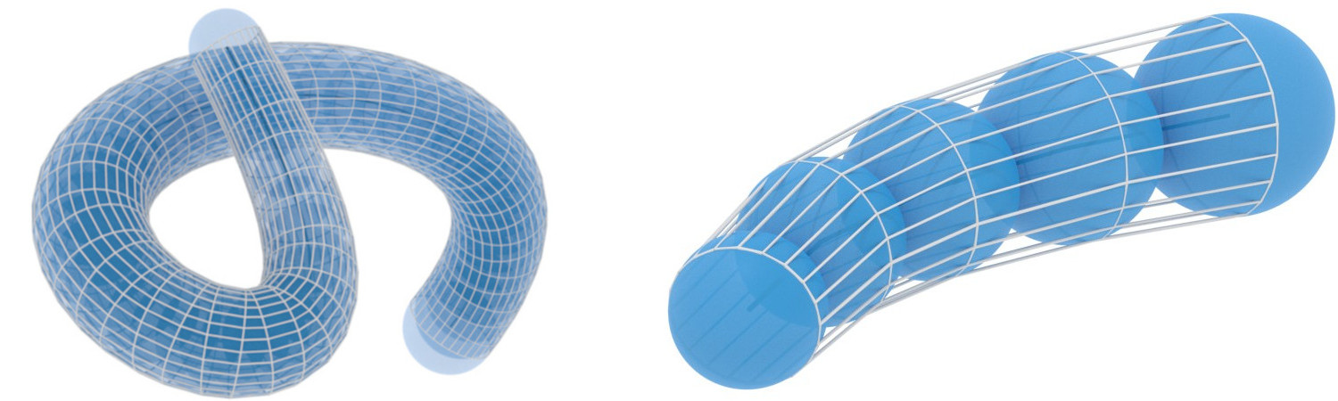
Channel Surfaces and Focal Surfaces

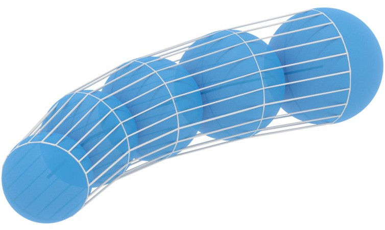
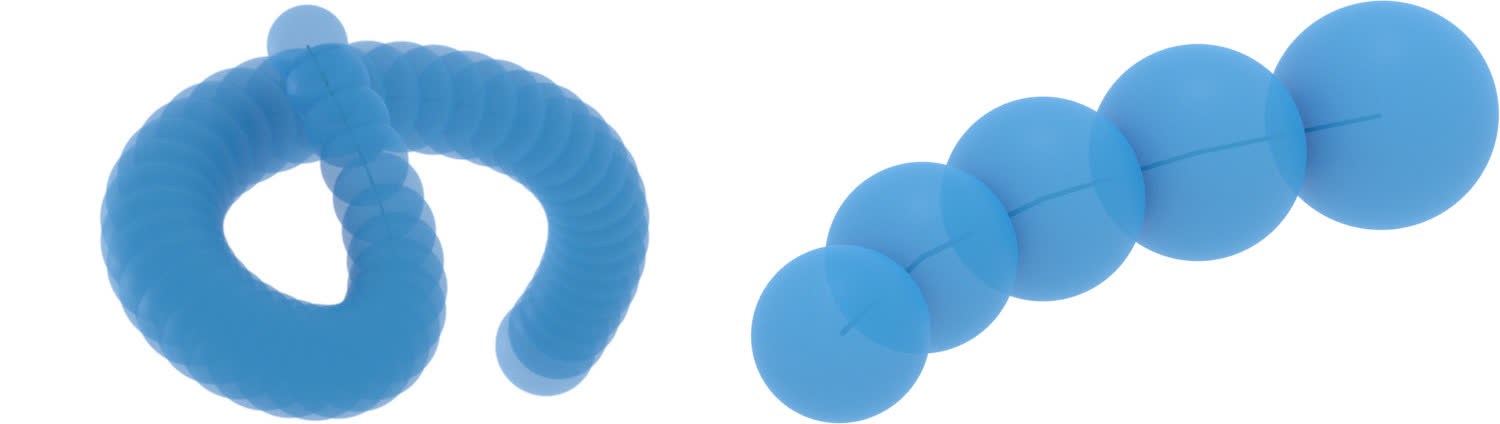
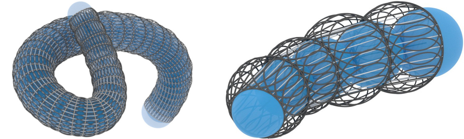
In this example we construct channel surfaces and focal surfaces. We start with a discrete one-parameter family of spheres. The channel surface can be obtained by choosing a circle on the first, or any, sphere and iteratively applying sphere inversions in the mid-spheres of anti-similitude. This will construct a discrete surface with planar, even circular faces. The circles can be used to define normal lines for the faces, the normal lines being orthogonal to the face and passing through the circles center. From the obtained normal line congruence we construct the two discrete focal surfaces by intersecting successive normal lines for each parameter direction. One of the focal surfaces degenerates to a discrete curve, which always is the case for channel surfaces. The main part of the example consists of a function taking as an argument a name for an example (smooth or discrete). We will go through the discrete example in this guide.

Download the full script here: channel_surfaces.py.

Very similar methods for sphere inversions and envelopes (in 2 dimensions) were introduced in the example Envelopes and Orthogonal Trajectories of Families of Circles. In some cases we will just refer to this example and refrain from detailed explanations here.

Setup

We start off by importing the necessary libraries, clearing the scene and initializing the projective and the Moebius geometric model of three dimensional Euclidean space.

# Import necessary libraries
import numpy as np

import ddg
from ddg.geometry.euclidean_models import moebius_to_projective, projective_to_moebius
from ddg.geometry.intersection import intersect, join
from ddg.geometry.subspaces import (
    Point,
    orthonormalize_and_center_subspace,
    subspace_from_affine_points,
)
from ddg.visualization.blender.material import material

# Clear the existing objects in the Blender scene
ddg.visualization.blender.scene.clear()
ddg.visualization.blender.material.clear()


euc = ddg.geometry.euclidean(3)
mob = ddg.geometry.euclidean_models.MoebiusModel(3)

The One-Parameter Family of Spheres

The main script starts by defining a lot of helper functions. In the end the examples will be generated only by suitable composition of these functions. A lot of the functions are straight forward, and we will not explicitly include all of them here. Furthermore, a lot of them have already been defined in the example on Envelopes and Orthogonal Trajectories of Families of Circles.

Now lets get started by defining a discrete curve in \(\mathbb{R}^3\), radii of spheres associated to the vertices and some initial values.

    elif example_name == "discrete":
        # Samplings in two parameter directions
        sampling_curve = 5
        v_circle_sampling = 20

        # Parameterization of a 2d parabola

        def parabola_parameterization(u):
            return 5 * np.array([u, -(u**2) / 2])

        snet_2d = ddg.nets.net.SmoothNet(
            parabola_parameterization, [[0, 1 / 2 * np.pi]]
        )
        snet = ddg.nets.utils.embed(snet_2d)
        dnet = ddg.sample_smooth_net(snet, sampling=[sampling_curve, "t"])

        # Radii of the spheres associated to the vertices
        radii = np.linspace(1, 2, sampling_curve)

        # Start of discrete envelope. The first circle is the intersection of this plane
        # with the first sphere
        plane = ddg.geometry.subspaces.Subspace(
            [-0.2, 1, 0, 1], [-0.2, 1, 1, 1], [-0.2, 0, 1, 1]
        )

        # Visualization domain of the focal surface
        domain_focal_surf = ddg.nets.DiscreteDomain([[0, 2], [-4, 3]])

        # Visualization
        dnet_bevel = 0.04
        camera_location = (-13, -5, 8)
        camera_look_at_point = (5, -2, 0)
    else:
        raise ValueError(
            "The only examples implemented are called 'smooth' and 'discrete'."
        )

We can define the one-parameter family of spheres as a discrete function and further, define their lift to homogeneous coordinates in \(\mathbb{R}^{4, 1}\) of the form \(\frac{1}{r}(c, \frac{1}{2}(||c||^2 - r^2 + 1) , \frac{1}{2}(||c||^2 - r^2 - 1))\).

    ###############################################
    # Spheres
    ###############################################

    # Euclidean ###################################
    def e_spheres_fct(i):
        return euc.sphere_from_affine_point_and_normals(dnet.fct(i), radii[i])

    # Moebius #####################################
    m_homogeneous_points_fct = homogeneous_lift_of_spheres_fct(
        e_spheres_fct
    )  # Homogeneous Points in R^{4, 1}

The Channel Surface

We can use the homogeneous coordinates to find the mid-spheres, in particular the spheres of anti-similitude (see Envelopes and Orthogonal Trajectories of Families of Circles).

    ###############################################
    # Spheres of anti-similitude
    ###############################################

    # Moebius #####################################
    m_points_of_anti_similitude_fct = (
        m_points_of_anti_similitude_from_homogeneous_lifts(m_homogeneous_points_fct)
    )  # Points in M+
    m_spheres_of_anti_similitude_fct = m_points_to_spheres(
        m_points_of_anti_similitude_fct
    )  # Quadrics in M

    # Euclidean ####################################
    e_spheres_of_anti_similitude_fct = project_function_of_objects_down(
        m_spheres_of_anti_similitude_fct
    )  # Spheres in R3

    ###############################################
    # Envelope (as sphere inversions in spheres of anti-similitude)
    ###############################################

    # Intersecting the first sphere with the plane (given in the initial values
    # of the example) determines a starting circle. A sampling yields a list of points.
    # Iterative sphere inversions in the mid-spheres of anti-similitude
    # form the discrete channel surface.

    # Starting circle ##############################
    circle = ddg.geometry.intersection.intersect(
        plane, euc.sphere_to_quadric(e_spheres_fct(0))
    )  # Conic in R3
    circle_dnet = ddg.sample_smooth_net(
        ddg.to_smooth_net(circle), sampling=[v_circle_sampling, "t"]
    )  # DiscreteNet in R3
    cirlce_pts = [
        circle_dnet.fct(k) for k, in circle_dnet.domain.traverser
    ]  # List of affine coordinates
    m_starting_pts = [
        projective_to_moebius(subspace_from_affine_points(p)) for p in cirlce_pts
    ]  # List of points in M

    # Moebius #####################################
    m_surface_points_fct = m_iterative_sphere_inversions(
        m_points_of_anti_similitude_fct, m_starting_pts
    )  # Two-parameter family of points in M

    # Euclidean ####################################
    e_surface_points_fct = function_projective_to_affine(
        project_function_of_objects_down(m_surface_points_fct)
    )  # Two-parameter family of affine coordinates

    def channel_surface_parameterization(i, j):
        return e_surface_points_fct(i)[j]

The visualization is also done by using helper functions and can be found as the last section of this guide.

Circumcircles and Normal Lines

    ###############################################
    # Circumcircles of the channel surface
    ###############################################

    # Channel surfaces are circular, for each face we determine the
    # circle through its four vertices. It suffices to determine the circle through
    # three of its vertices.
    def face_circles_data(i, j):
        """
        Returns the center, radius, and normal of the
        circumcircle of the face [(i, j), (i+1, j), (i+1, j+1), (i, j+1)].
        """
        points = [
            channel_surface_parameterization(i, j),
            channel_surface_parameterization(i + 1, j),
            channel_surface_parameterization(i, j + 1),
        ]
        c, r, n = ddg.math.euclidean.circle_through_three_points(*points)
        return c, r, n

    def face_circles(i, j):
        """
        Returns the circumcircle of the face [(i, j), (i+1, j), (i+1, j+1), (i, j+1)].
        """
        return euc.sphere_from_affine_point_and_normals(*face_circles_data(i, j))

    ##############################################
    # Normal line congruence
    ##############################################
    # From the same data we can compute face normal lines,
    # orthogonal to the faces and passing through the centers
    # of the circumcircles.
    def normal_line_congruence(i, j):
        """
        Returns the normal line to each face passing through the circumcircles center.
        """
        c, r, n = face_circles_data(i, j)
        line = ddg.geometry.subspaces.subspace_from_affine_points_and_directions(c, n)
        return line

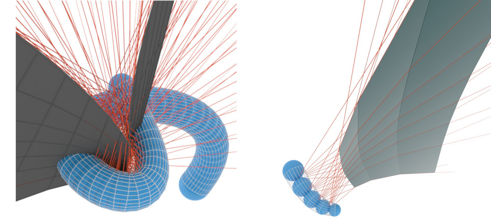
For each parameter line in the first parameter direction the corresponding circles lie on a sphere, the curvature sphere (nicely to see in the right picture below). All the normal lines corresponding to this family in the first parameter direction pass through the spheres center.

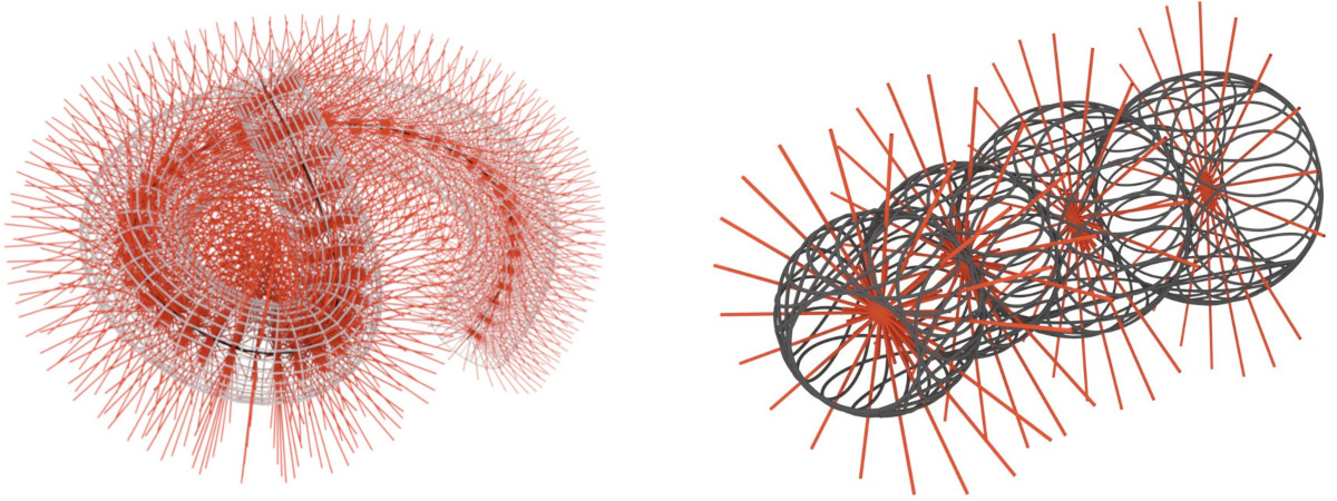
The Focal Surfaces

    ##############################################
    # Focal surfaces
    ##############################################

    # Neighbouring normal lines intersect. The intersection points
    # determine two new surfaces, the focal surfaces.
    # One of these surfaces degenerates to a discrete curve. We compute the other.

    def focal_surf_i(i, j):
        """
        Returns the intersection points of successive normal lines in the fist
        parameter direction.
        """
        return ddg.geometry.intersection.intersect(
            normal_line_congruence(i, j), normal_line_congruence(i + 1, j)
        ).affine_point

Visualization

With all this setup done, we can now visualize this in Blender. We start by defining some colors and helper functions. For some functions the discrete domain may be clipped at the start or at the end. For this we also use a helper function.

################################################
# Visualization setup
################################################
orange = material("orange", (0.8, 0.1, 0.036), 0, 0)
gray = material("gray", (0.1, 0.1, 0.1), 0, 0, 1)
black = material("black", (0, 0, 0), 0, 0, 1)
lightgray = material("lightgray", (0.7, 0.7, 0.7), 0, 0, 1)
transparent_sphere = ddg.visualization.blender.material.material(
    "transparent_sphere", (0.018, 0.313, 0.656), 0.5, 0.5, alpha=0.8
)

bevel = 0.03
sampling = [0.1, 100, "c"]


def visualize_spheres(g, domain, **kwargs):
    return [
        ddg.to_blender_object_helper(
            g(i),
            sampling=sampling,
            name=f"sphere_{i}",
            **kwargs,
        )
        for i, in domain.traverser
    ]


def visualize_lines(g, domain, line_domain, **kwargs):
    return [
        ddg.to_blender_object_helper(
            g(i, j),
            domain=line_domain,
            sampling=sampling,
            curve_properties={"bevel_depth": bevel},
            name=f"line_{i}",
            **kwargs,
        )
        for i, j in domain.traverser
    ]


def visualize_circles(g, domain, **kwargs):
    return [
        ddg.to_blender_object_helper(
            g(i, j),
            sampling=sampling,
            curve_properties={"bevel_depth": bevel},
            name=f"circle_{i}",
            **kwargs,
        )
        for i, j in domain.traverser
    ]


def wire_bobj_to_curve(bobj, bevel_depth=0.025):
    # Choose the object mode context
    with ddg.visualization.blender.context.mode(bobj, mode="OBJECT"):
        # Save the material
        mat = bobj.active_material
        # Select the object
        bpy.ops.object.select_all(action="DESELECT")
        bobj.select_set(True)
        # Convert it to a curve
        bpy.ops.object.convert(target="CURVE")
        # Unselect the object
        bobj.select_set(False)
        # Set its bevel_depth and its material
        bobj.data.bevel_depth = bevel_depth
        ddg.visualization.blender.material.set_material(bobj, mat)
        return bobj

For each example (“smooth”/”discrete”) we add a set of collections …

    col = ddg.visualization.blender.collection.collection(
        f"Channel_surface_{example_name}",
        children=[
            f"spheres_{example_name}",
            f"envelope_{example_name}",
            f"circumscribed_circles_{example_name}",
            f"normal_lines_{example_name}",
            f"focal_surfaces_{example_name}",
        ],
    )

… and visualize all the objects.

    ###############################################
    # Channel surface
    ###############################################

    # Discrete curve
    ddg.to_blender_object_helper(
        dnet, curve_properties={"bevel_depth": dnet_bevel}, material=black
    )
    # Spheres
    visualize_spheres(
        e_spheres_fct,
        domain=dnet.domain,
        material=transparent_sphere,
        collection=col.children[0],
    )

    # Channel surface
    channel_surface_domain = ddg.nets.DiscreteDomain(
        [dnet.domain[0], [0, v_circle_sampling - 1, True]]
    )
    channel_bobj = ddg.to_blender_object_helper(
        ddg.nets.DiscreteNet(
            channel_surface_parameterization,
            domain=channel_surface_domain,
        ),
        material=lightgray,
        only_wire=True,
        collection=col.children[1],
    )

    wire_bobj_to_curve(channel_bobj)

    ###############################################
    # Circumscribed circles
    ###############################################
    circumcircles_domain = ddg.nets.DiscreteDomain(
        [[dnet.domain[0][0], dnet.domain[0][1] - 1], [0, v_circle_sampling - 2]]
    )
    visualize_circles(
        face_circles,
        domain=circumcircles_domain,
        material=gray,
        collection=col.children[2],
    )

    ###############################################
    # Normal line congruence
    ###############################################

    visualize_lines(
        normal_line_congruence,
        domain=circumcircles_domain,
        line_domain=[[-2, 2]],
        material=orange,
        collection=col.children[3],
    )

    ###############################################
    # Focal surface
    ###############################################

    visualize_lines(
        normal_line_congruence,
        domain=domain_focal_surf,
        line_domain=[[0, 100]],
        collection=col.children[4],
        material=orange,
    )

    focal_dnet = ddg.DiscreteNet(focal_surf_i, domain=domain_focal_surf)
    ddg.to_blender_object_helper(focal_dnet, material=gray, collection=col.children[4])
    focal_wire = ddg.to_blender_object_helper(
        focal_dnet, only_wire=True, material=gray, collection=col.children[4]
    )
    wire_bobj_to_curve(focal_wire, bevel_depth=0.04)

The script further includes adding lights and cameras and setting up the scene for rendering.