Envelope, Evolute, Orthogonal Trajectory and Involute of Curves
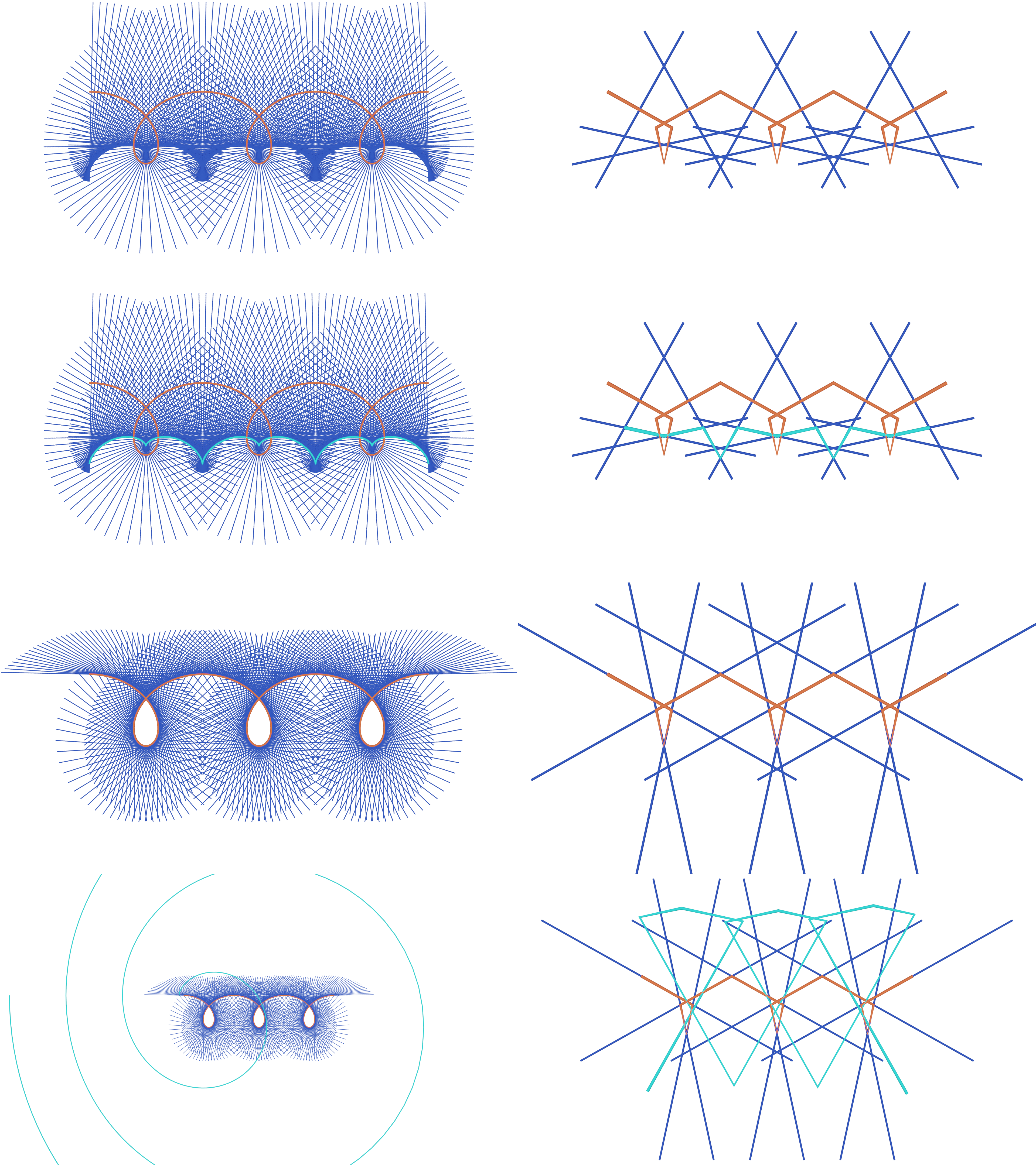
In this example we will generate the following
(from top to bottom in the above picture),
a curve with its edge normals, a curve with its edge normals and its evolute,
a curve with its tangent lines,
a curve with its tangent lines and an involute.
The left side shows a fine sampling of a smooth curve,
the right side a sparse sampling.
You can see the full code at
involute_evolute_curve.py.
Setup
We start off by importing the necessary libraries.
# Import necessary libraries
import numpy as np

import ddg
from ddg.geometry.intersection import intersect
from ddg.geometry.subspaces import (
    angle_bisector_orientation_reversing,
    level,
    normal,
    orthonormalize_and_center_subspace,
    perpendicular_bisector,
    subspace_from_affine_points,
)
from ddg.math.euclidean import reflection_in_a_hyperplane
from ddg.math.projective import dehomogenize, homogenize
from ddg.visualization.blender.material import material
We are also going to clear the whole scene.
# Clear the existing objects in the Blender scene
ddg.visualization.blender.scene.clear()


ddg.visualization.blender.material.clear()
General Functions
Now we are going to define functions that will generate edge tangent
lines, vertex normal lines and edge normal lines for a discrete
curve given by a function fct.
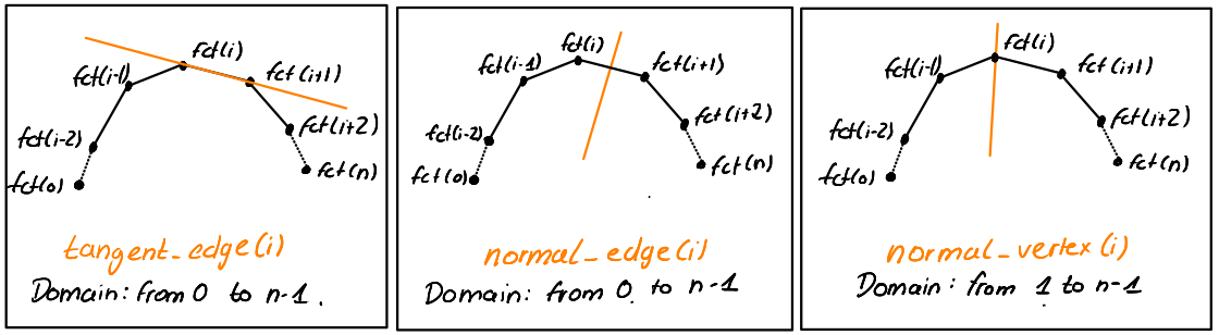
def tangent_edges(fct):
    """Returns a function that, for a given index,
    returns the edge tangent line with given index of the
    discrete curve in the input.
    The i'th edge tangent line is the join of fct(i) and fct(i+1).
    """

    @lru_cache(maxsize=128)
    def tangent_edge(i):
        tangent = subspace_from_affine_points(fct(i), fct(i + 1))
        return orthonormalize_and_center_subspace(
            tangent, np.sum([fct(i), fct(i + 1)], axis=0) / 2
        )

    return tangent_edge


def normal_edges(fct):
    """Returns a function that, for a given index,
    returns the edge normal line with given index of the
    discrete curve in the input.
    The i'th edge normal line is the perpendicular
    bisector of fct(i) and fct(i+1).
    """

    @lru_cache(maxsize=128)
    def normal_edge(i):
        normal = perpendicular_bisector(
            subspace_from_affine_points(fct(i)), subspace_from_affine_points(fct(i + 1))
        )
        return orthonormalize_and_center_subspace(
            normal, np.sum([fct(i), fct(i + 1)], axis=0) / 2
        )

    return normal_edge


def normal_vertices(fct):
    """Returns a function that, for a given index,
    returns the vertex normal line with given index of the
    discrete curve in the input.
    The i'th vertex normal line is the orientation reversing
    angle bisector of the (i-1)'st and i'th edge tangent line.
    """

    @lru_cache(maxsize=128)
    def normal_vertex(i):
        normal = angle_bisector_orientation_reversing(
            tangent_edges(fct)(i - 1), tangent_edges(fct)(i)
        )
        return orthonormalize_and_center_subspace(normal, fct(i))

    return normal_vertex
Next we define a function returning the envelope (as a function) for a given family of lines. The envelope is a new curve consisting on intersection points of successive lines. Also we define a function returning the orthogonal_trajectory (as a function) for a given family of lines and a starting point. The orthogonal trajectory is the iterative reflection of a starting point on the lines of the line family.
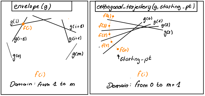
def envelope(g):
    """The return value of the function g is assumed to be a line.
    Then this function returns a function that, for a given index i,
    returns the intersection of the (i-1)'st and i'th
    line of g.
    """

    @lru_cache(maxsize=128)
    def new_curve_fct(i):
        point = intersect(g(i - 1), g(i))
        return point.affine_point

    return new_curve_fct


@lru_cache(maxsize=128)
def orthogonal_trajectory(g, starting_point):
    """The return value of the function g is assumed to be a line.
    Then this function returns a function that, for a given index i,
    returns the i'th iterative reflection of the starting point
    on the first i lines of g.
    Example: new_curve_fct(0) returns the starting_point,
    new_curve_fct(1) returns the starting point reflected on the
    line g(0), new_curve_fct(2) returns the point new_curve_fct(1)
    reflected on the line g(1).
    """

    @lru_cache(maxsize=128)
    def new_curve_fct(i):
        if i == 0:
            return starting_point
        else:
            n, l = normal(g(i - 1)), level(g(i - 1))
            return dehomogenize(
                reflection_in_a_hyperplane(n, l) @ homogenize(new_curve_fct(i - 1))
            )

    return new_curve_fct
Example
Next we set values for the example images at the top. Feel free to experiment with this or change the curve we have chosen in this example. Choosing a starting point for the involute to look nice might be quite tricky.
example = "smooth"
if example == "smooth":
    sampling_curve = np.pi / 50
    bevel_curve = 0.05
    bevel_line = 0.02
    involute_start = (-10, 3)
    edge_domain = [[-5, 5]]
if example == "discrete":
    sampling_curve = np.pi / 2
    bevel_curve = 0.1
    bevel_line = 0.06
    involute_start = (-9, -5)
    edge_domain = [[-10, 10]]
Then we define our parametrized curve.
# We define a parametrization for a curve.
a, b = 1, 2


def parametrization(u):
    return [a * u - b * np.sin(u), a * 1 - b * np.cos(u)]


# We set a definition domain and initialize the smooth curve.
smooth_domain = [[-3 * np.pi, 3 * np.pi]]
snet = ddg.nets.SmoothNet(parametrization, domain=smooth_domain)
Now we can create a discrete net by sampling the smooth net.
# Define a sampling and initialize the discrete curve.
# The domain of the discrete curve is [[0, d]],
# where d is the number of steps in the smooth domain
# determined by the sampling.
dnet = ddg.sample_smooth_net(snet, sampling=sampling_curve)
Now we can use the previously defined functions to create functions that generate edge tangent lines, vertex normal lines and edge normal lines for our curve. Further these can be used to create evolutes and involutes: The envelope of tangent lines of a curve is its evolute, the orthogonal trajectory of a starting point along normal lines of a curve forms an involute.
# Define edge tangent line, vertex normal line and edge normal line
# functions for the given curve.
tangent_edge = tangent_edges(dnet.fct)
normal_edge = normal_edges(dnet.fct)
normal_vertex = normal_vertices(dnet.fct)

# Define evolutes for edge normal lines and vertex normal lines and
# an involute for the edge tangent lines.
evolute_vertex = envelope(normal_edge)
evolute_edge = envelope(normal_vertex)
involute = orthogonal_trajectory(tangent_edge, involute_start)
We can compute the envelope of the normal lines of the involute, i.e. the evolute of the involute. This will yield the curve we have started with.
# Define normals of the involute.
normal_edge_involute = normal_edges(involute)

# Define the evolute of the normals of the involute.
evolute_involute_edge = envelope(normal_edge_involute)
Visualization
With all this setup done, we can now visualize this in Blender. We start by defining some colors and a helper function. For the normal or tangent line functions, and thus also the envelopes and orthogonal trajectories, the domain of the newly generated functions may be clipped at the start or at the end. For this we use this helper function.
orange = material("orange", (0.8, 0.1, 0.036), 0, 0)
blue = material("blue", (0.019, 0.052, 0.445), 0, 0)
turquoise = material("turquoise ", (0.02, 0.8, 0.77), 0, 0)


def shift_domain(a, b):
    return [[dnet.domain[0][0] + a, dnet.domain[0][1] + b]]
Next we will define helper functions for the visualization.
The first function takes a function as an input that returns the
2d coordinates of a curve. The helper function converts the input to
an actual curve and embeds it into 3d space, namely in the z=0 plane,
such that it can be visualized in Blender.
The second helper function takes a function as an input,
that returns lines in 2d space, represented as subspaces.
This helper function visualizes all the lines of the input function
(in the given domain) by also embedding them into the z=0 plane.
For nets and subspace the embed functions are different.
def visualize_2d_curve(dnet_fct, domain=dnet.domain, **kwargs):
    dnet = ddg.nets.DiscreteNet(dnet_fct, domain=domain)
    return ddg.to_blender_object_helper(
        ddg.nets.utils.embed(dnet),
        material=orange,
        curve_properties={"bevel_depth": bevel_curve},
        **kwargs,
    )


def visualize_2d_lines(g, domain=dnet.domain, line_domain=[[-5, 5]], **kwargs):
    return [
        ddg.to_blender_object_helper(
            g(i).embed(),
            sampling=1,
            domain=line_domain,
            curve_properties={"bevel_depth": bevel_line},
            material=blue,
            name=f"g_{i}",
            **kwargs,
        )
        for i in range(*domain[0])
    ]
Using the helper functions, we visualize the curves and lines in Blender.
bobj = visualize_2d_curve(dnet.fct, name="Discrete Curve")

visualize_2d_lines(normal_edge)
evolute_edge_bobj = visualize_2d_curve(
    evolute_edge, domain=shift_domain(1, -1), name="Evolute_edge"
)

visualize_2d_lines(normal_vertex, shift_domain(1, 0))
evolute_vertex_bobj = visualize_2d_curve(evolute_vertex, name="Evolute_vertex")

visualize_2d_lines(tangent_edge, line_domain=edge_domain)
involute_bobj = visualize_2d_curve(involute, name="Involute")

visualize_2d_lines(normal_edge_involute, line_domain=[[-10, 10]])
evolute_involute_edge_bobj = visualize_2d_curve(
    evolute_involute_edge, domain=shift_domain(1, -1), name="Evolute of Involute"
)
Finally we need to add a camera and a light to our scene and set the render mode.
# Add a point light and a camera to the scene
light = ddg.visualization.blender.light.light(
    location=(0, 0, 100), type_="SUN", energy=5
)
camera = ddg.visualization.blender.camera.camera(location=(0, 0, 40))
ddg.visualization.blender.render.setup_cycles_renderer()
ddg.visualization.blender.render.set_film_transparency()