Elliptic Billiard

This example illustrates the elliptic billiard. Given an ellipse, we trace the trajectory of a particle moving with constant velocity in its interior and reflecting in its boundary. The reflections are specular: the angle of reflection equals the angle of incidence.

Using our library, we will write an interactive script to visualize the trajectories starting from any point on an ellipse. You can find the full script here elliptic-billiards.py.

Setup

To set up our scene, we create an ellipse and use its parameterization function to define an arbitrary chord. This is equivalent to choosing a point on the ellipse and a direction to begin the trajectory.

    # Choose major and minor axes of the ellipse with a > b.
    a = 3.5
    b = 1.0
    # Create the ellipse and its parameterization.
    ellipse = Quadric(np.diag([1 / a, 1 / b, -1]))
    ellipse_snet = ddg.to_smooth_net(ellipse.embed())
    ellipse_parameterization = ellipse_snet.fct
    ellipse_dnet = ddg.sample_smooth_net(ellipse_snet, [0.006, 300, "c"])

    # A chord is determined by two points on the ellipse.
    # We choose the initial chord using parameterization function of ellipse.
    # Set t0 and t1 accordingly.
    epsilon = 0.1
    t0 = np.pi / 2 - epsilon
    t1 = 3 * np.pi / 2 + epsilon

    s0 = ellipse_parameterization(t0)[:-1]
    s1 = ellipse_parameterization(t1)[:-1]

    # The queue stores the points of the billiard map as ddg.Point's.
    queue = [Subspace(homogenize(s0)), Subspace(homogenize(s1))]

Billiard map

We define our main billiard map. It takes the chord joining a start and an end point along the trajectory and reflects it in the line, tangent to the ellipse at the end point.

def billard_map(conic, incidence_chord):
    """
    Returns a reflected point given incidence chord of a conic.

    Parameters
    ----------
    conic : ddg.geometry.quadrics.Quadric
        A conic in projective space.
    incidence_chord : Tuple of two ddg.geometry.subspaces.Subspace.Point
        A chord defined by two points on conic.

    Returns
    -------
    ddg.geometry.subspaces.Subspace.Point
    """
    p0, p1 = incidence_chord
    chord_subspace = join_subspaces(p0, p1)

    # Get tangent line to conic at p1.
    tangent_subspace = polarize(p1, conic)

    assert p1 in conic
    assert p1 in tangent_subspace

    # Reflect the chord in the tangent line.
    reflected_chord = reflect_in_hyperplane(chord_subspace, tangent_subspace)
    # Get other intersection point with conic.
    intersection_points = intersect_quadric_subspace(conic, reflected_chord)
    p, q = quadric_to_subspaces(intersection_points)
    if p == p1:
        reflected_point = q
    else:
        reflected_point = p

    return reflected_point

Visualization

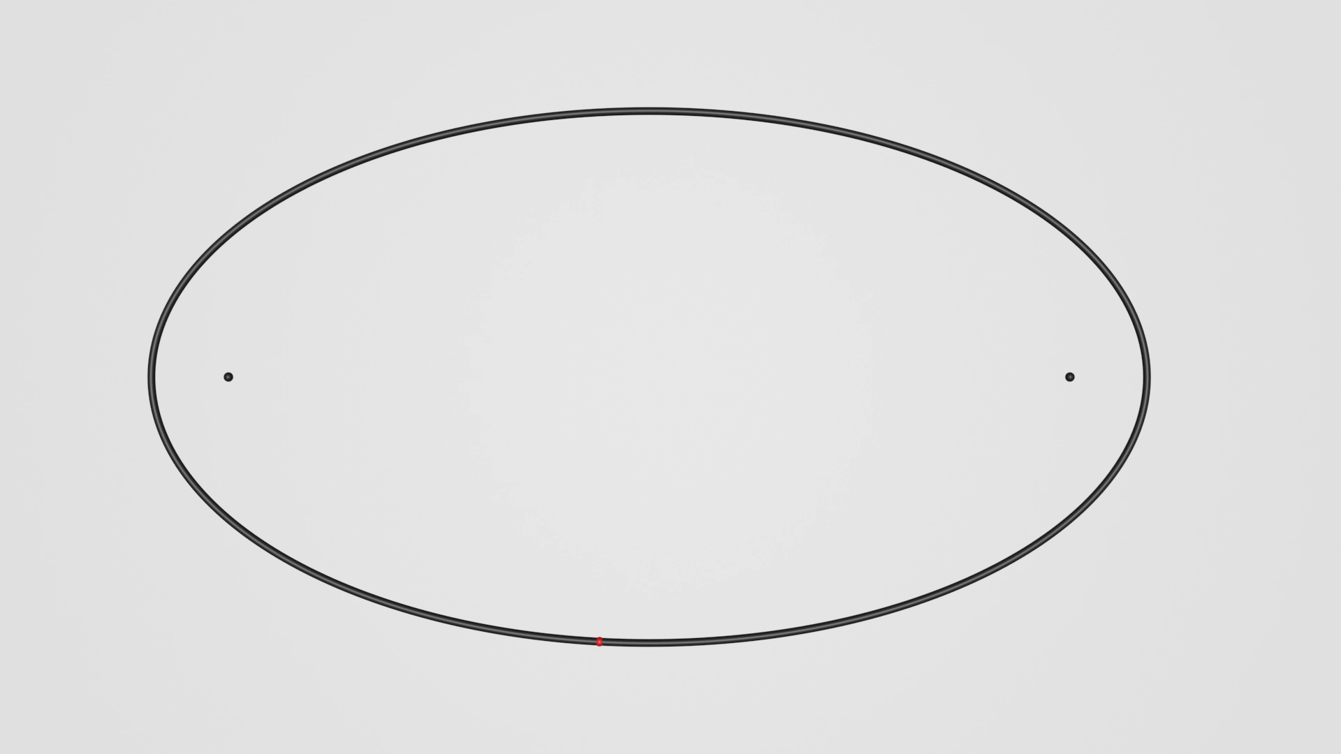
At this stage, we can visualize the static objects, namely the ellipse and its focal points. We also define materials, and add a top light and a camera.

    # -------------
    # Visualization
    # -------------

    # Set size for visualized points.
    points_size = 0.018
    # Set thickness of visualized curves.
    chord_thickness = 0.004
    ellipse_thickness = 0.015

    # Setup camera.
    camera = camera(name="top_camera", location=(0.0, 0.0, 7.0), collection=static_col)

    # Setup light.
    light = light(name="top_light", type_="SUN", energy=2.0, collection=static_col)

    # Setup basic materials.
    point_material = material("point_material", color=(1.0, 0.0, 0.0))
    chord_material = material("line_material", color=(0.0, 0.130, 0.717))
    ellipse_material = material("ellipse_material", color=(0.015, 0.015, 0.015))

    # Visualize ellipse.
    ddg.to_blender_object(
        ellipse_dnet,
        material=ellipse_material,
        attributes={"name": "ellipse"},
        curve_properties={"bevel_depth": ellipse_thickness},
        collection=static_col,
    )
    # Define and visualize its focal points.
    f1 = Subspace([np.sqrt(a - b), 0.0, 0.0, 1.0])
    f2 = Subspace([-np.sqrt(a - b), 0.0, 0.0, 1.0])
    ddg.to_blender_object_helper(
        f1,
        name="first_focal_point",
        sphere_radius=points_size,
        material=ellipse_material,
        collection=static_col,
    )
    ddg.to_blender_object_helper(
        f2,
        name="second_focal_point",
        sphere_radius=points_size,
        material=ellipse_material,
        collection=static_col,
    )

Add interactive property

Here we set the maximum number of reflections

    N = 50

and assign the current number of reflections as a custom property to our scene

    ddg.visualization.blender.props.add_props_with_callback(run_step, ("i"), 0)

We define the callback function run_step

def run_step(i):
    # The animation is designed to iteratively run through the steps.
    if len(queue) < i:
        warnings.warn(
            f"Attempted billiards iteration {i} "
            "before calling the previous iterations. "
            "Please run them in order."
        )
        return None

    else:
        p0 = queue[i - 2]
        p1 = queue[i - 1]

        # 1st step: Clear animated objects and visualize 0'th point.
        if i == 1:
            clear(collections=[animated_col])
            ddg.to_blender_object_helper(
                p1.embed(),
                sphere_radius=points_size,
                material=point_material,
                collection=animated_col,
            )

        # When running the animation the fist time new points have to be generated.
        if len(queue) == i:
            reflected_point = billard_map(ellipse, (p0, p1))
            queue.append(reflected_point)

        # When running the animation multiple times points in the queue can be accessed.
        elif len(queue) > i:
            reflected_point = queue[i]

    # New chord generated by reflection.
    chord = join_subspaces(p1, reflected_point)

    # Embed and visualize the new point and the new chord line.
    ddg.to_blender_object_helper(
        reflected_point.embed(),
        sphere_radius=points_size,
        material=point_material,
        collection=animated_col,
    )
    ddg.to_blender_object_helper(
        chord.embed(),
        domain=[[0, 1]],
        sampling=[0.006, 300, "c"],
        curve_properties={"bevel_depth": chord_thickness},
        material=chord_material,
        collection=animated_col,
    )

Animation and Rendering

To create an animation, one can set keyframes as shown:

    set_keyframe(scene, 1, "i", 1)
    set_keyframe(scene, N, "i", N)

To render it, we can use the function ddg.visualization.blender.render.render_animation() after setting the render settings

    # Setup render settings
    output_dir = "/"
    scene.render.fps = 4
    scene.view_settings.view_transform = "Standard"
    setup_eevee_renderer(scene=scene)
    set_film_transparency(scene=scene)
    set_render_output_images(output_dir, time=False)

It’s also possible to add a render stamp beforehand, as shown:

    # Display render stamp of parameters.
    parameters_string = " N = " + str(N)
    parameters_string += "\n a = " + np.format_float_positional(a, precision=3)
    parameters_string += "\n b = " + np.format_float_positional(b, precision=3)
    parameters_string += "\n t₀ = " + np.format_float_positional(t0, precision=3)
    parameters_string += "\n t₁ = " + np.format_float_positional(t1, precision=3)
    set_render_stamp_note(note=parameters_string, scene=scene)

    # Do not display any other render stamp.
    scene.render.use_stamp_date = False
    scene.render.use_stamp_time = False
    scene.render.use_stamp_frame = False
    scene.render.use_stamp_scene = False
    scene.render.use_stamp_labels = False
    scene.render.use_stamp_camera = False
    scene.render.use_stamp_filename = False
    scene.render.use_stamp_render_time = False