Shadow of a Quadric

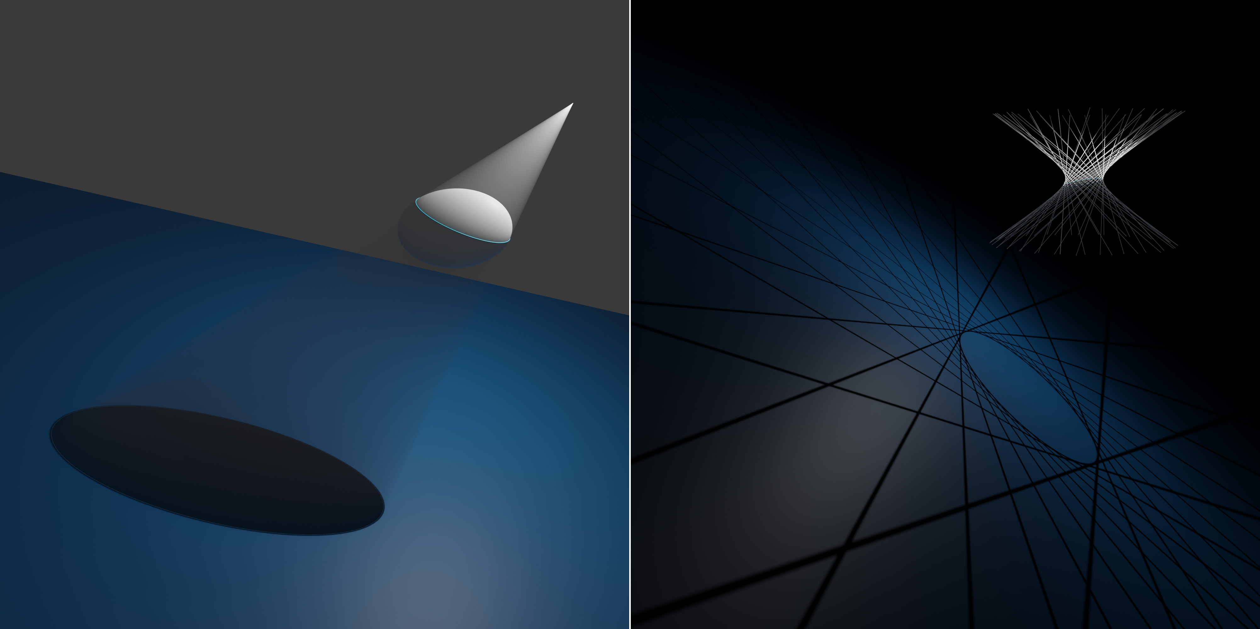
This example visualizes the shadow of a quadric cast by a light source. You can see the full code at shadow_of_a_quadric.py.

Setup

We start off by importing the necessary libraries.

# Import necessary libraries and modules
import numpy as np

import ddg
import ddg.geometry as geo
from ddg.geometry.intersection import intersect
from ddg.math.projective import dehomogenize, homogenize
from ddg.visualization.blender.scene import clear

We are also going to clear the whole scene.

# Clear the Blender scene
clear()

Constants

Now we are going to define some constants that we will use later. In particular the data for the images above is given below.

# example, visualize_generators = 'ellipsoid', False
example, visualize_generators = "one_sheeted_hyperboloid", True

# Define parameters for the quadric, the location of the light source
# and the normal and level of the projection plane
if example == "ellipsoid":
    a, b, c, d = 4, 0.5, 1, -2
    light_x, light_y, light_z = 1, 4, 4
    normal_x, normal_y, normal_z, level = 3, 1, 4, -10
if example == "one_sheeted_hyperboloid":
    a, b, c, d = 1, 0.5, -1, -1
    light_x, light_y, light_z = 1, 1.2, 4
    normal_x, normal_y, normal_z, level = 3, 1, 4, -15

# Define the position of the light source and normalize the planes
# normal
light = np.array([light_x, light_y, light_z])
normal_tmp = np.array([normal_x, normal_y, normal_z])
normal = normal_tmp / np.linalg.norm(normal_tmp)

Further define constants for sampling and visualization.

# Sampling for Blender objects
quadric_sampling = [0.1, 100, "c"]
projection_plane_sampling = [1, 100, "c"]
polar_plane_sampling = [1, 100, "c"]
polar_plane_intersection_sampling = [1, 100, "c"]
t_cone_sampling = [0.1, 100, "c"]
projection_sampling = [0.03, 100, "c"]

if example == "ellipsoid":
    bounding_box_for_projection_plane = np.array([15, 25, 25])
    camera_loc, camera_look_at = [31, 0, -5], [0, -5, -3]

if example == "one_sheeted_hyperboloid":
    bounding_box_for_projection_plane = 5 * np.array([15, 25, 25])
    camera_loc, camera_look_at = [18, -65, 10], [0, 0, -5]

if visualize_generators:
    density_of_generators = 1 / 12 * np.pi
    generators_sampling = 0.1
    generators_bounding_box = [100, 100, 5]

Main Construction

Now we can begin with the actual construction of this visualization. First of all we need a quadric that we create from our initial data. For this example we restrict to quadrics with diagonal matrix.

# Create a quadric
quadric = geo.quadrics.Quadric(np.diag([a, b, c, d]))

Next, let’s create the touching cone (or tangent cone) to the quadric from the light source. This is the join of all lines through the point of the light source that are tangent to the quadric, see also Quadrics.

# Construct the touching cone of the light source w.r.t. the quadric
t_cone = geo.quadrics.touching_cone(homogenize(light), quadric)
t_cone = t_cone.normalize(affine=True)

The points where the tangent cone touches the quadric can be determined explicitely. They are given by the intersection of the polar plane of the point of the light source with the quadric.

# Create a polar plane and find its intersection with the quadric
light_p = geo.subspaces.Point(homogenize(light))
polar_plane = geo.quadrics.polarize(light_p, quadric)
intersection = intersect(polar_plane, quadric)

Finally we create a projection plane and can explicitly determine the boundary of the shadow by intersecting the tangential cone with the projection plane.

# Create a projection plane
projection_plane = geo.subspaces.hyperplane_from_normal(normal, level=level)
# Intersect the touching cone and the projection plane
projection = intersect(t_cone, projection_plane)

Visualization

With all this we can now visualize everything in Blender. Note that we have not assigned materials in this example.

We start with the quadric and, for the one-sheeted hyperboloid example, its generators. The generators are determined in the following way. Take a conic section of the hyperboloid, for example the intersection with the polar plane from above. Convert it to a (SmoothNet and then to a) DiscreteNet using a rational multible of np.pi as a sampling. This gives a uniform, closed sampling of points on the conic section. One can use a traverser to iterate through the domain of the discrete curve an thus through the points on the conic. The polar plane of a (projective) point x on the conic is the tangent plane at x and intersects the hyperboloid in two generators, meeting in x. These we can visualize.

# Create a Blender object for the quadric
quadric_bobj = ddg.to_blender_object_helper(
    quadric,
    shade_smooth=True,
    sampling=quadric_sampling,
    bounding_box=[None, None, 5],
    material="quadric",
    name="quadric",
)
# Visualize the generators if necessary
if visualize_generators:
    discrete_intersection = ddg.sample_smooth_net(
        ddg.to_smooth_net(intersection), density_of_generators
    )
    generators = [
        intersect(
            quadric,
            geo.quadrics.polarize(
                geo.subspaces.subspace_from_affine_points(discrete_intersection.fct(i)),
                quadric,
            ),
        )
        for i, in discrete_intersection.domain.traverser
    ]
    generator_bobjs = [
        ddg.to_blender_object_helper(
            g,
            sampling=generators_sampling,
            bounding_box=generators_bounding_box,
            material="quadric_emission",
            name="generator",
        )
        for g in generators
    ]

Next, we will create a camera and a light source. The light sits at the apex of the touching cone and we let it shine parallel to the axis of the cone.

# Create a camera
camera_bobj = ddg.visualization.blender.camera.camera(location=camera_loc)
ddg.visualization.blender.camera.look_at_point(camera_bobj, camera_look_at)
# Create a light
light_bobj = ddg.visualization.blender.light.light(type_="SPOT", location=light)
if example == "ellipsoid":
    # Rotate the light source to match the touching cone orientation
    axis = ddg.geometry.quadrics.axis(t_cone)
    two_points = ddg.geometry.conversion.quadric_to_subspaces(
        ddg.geometry.intersection.intersect(quadric, axis)
    )
    ddg.visualization.blender.light.look_at_point(
        light_bobj, two_points[0].affine_point
    )
# Set light properties
light_bobj.data.spot_size = np.pi
light_bobj.scale *= 10
light_bobj.data.energy = 4000
light_bobj.data.spot_blend = 0
light_bobj.data.shadow_soft_size = 0.01

Now we are going to visualize one half of the cone.

# Create a tangent cone
t_cone_snet = ddg.to_smooth_net(t_cone)
t_cone_snet.domain.intervals[1] = [0, 200]
t_cone_dnet = ddg.sample_smooth_net(t_cone_snet, sampling=t_cone_sampling)
t_cone_bobj = ddg.to_blender_object_helper(
    t_cone_snet, sampling=t_cone_sampling, material="tcone", name="touching_cone"
)

The next step is to add the projection plane and the boundary of the shadow.

# Projection plane and intersection
center = intersect(
    geo.subspaces.subspace_from_affine_points(np.array([0, 0, 0]), light),
    projection_plane,
)
projection_plane_centered = projection_plane.center(center)
bb_trafo = lambda bmesh: ddg.visualization.blender.bmesh.cut_bounding_box(
    bmesh, bounding_box_for_projection_plane, dehomogenize(center.point)
)
projection_plane_bobj = ddg.to_blender_object_helper(
    projection_plane_centered,
    sampling=projection_plane_sampling,
    material="projection_plane",
    name="projection_plane",
    bmesh_transformations=[bb_trafo],
)
projection_bobj = ddg.to_blender_object_helper(
    projection, sampling=projection_sampling, material="projection", name="projection"
)

And finally, we create the polar plane and its intersection.

# Polar plane and intersection
polar_plane_orth = ddg.geometry.subspaces.orthonormalize_subspace(polar_plane)
polar_plane_bobj = ddg.to_blender_object_helper(
    polar_plane_orth,
    sampling=polar_plane_sampling,
    material="polar_plane",
    name="polar_plane",
)

polar_plane_intersection_bobj = ddg.to_blender_object_helper(
    intersection,
    sampling=polar_plane_intersection_sampling,
    material="polar",
    name="shadow_line",
    bounding=500,
)